Petrophysics Software - JLog® Version 11
JLog is affordable petrophysics software for individuals, consultants, independents and small companies that need to do well log analysis from time to time. Consultants have paid for JLog with their first job. JLog is easy to use and install. There is no annual support fee or maintenance fee or yearly membership fee.
The JLog author has been working with logs for over 50 years and has been developing petrophysical software since 1986. JLog has been under continuous development since 2000 and has been shipped to customers in 30 countries.
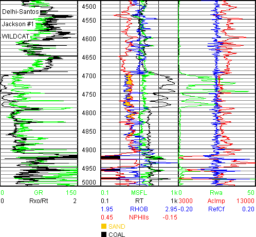
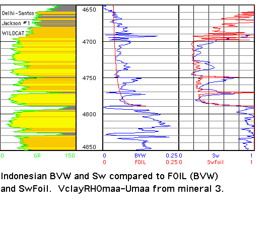
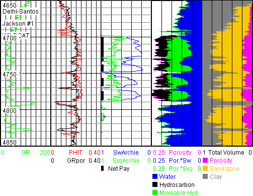
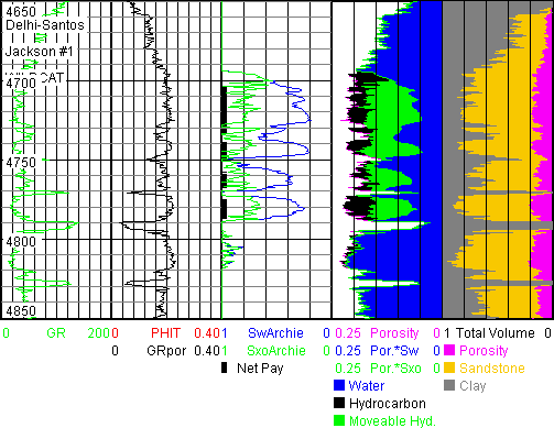
JLog is designed to quantify hydrocarbons in place for conventional and identify hydrocarbons, and in some cases, quantify hydrocarbons in unconventional reservoirs including source rock. Data and answers can be exported and saved in LAS, TEXT and graphic file formats. This makes it possible to generate all digital reports with common, off-the-shelf, software. The www.jlog.biz website (doubles as JLog User Manual) graphics are mostly JLog GIF files, as below, and screen shots.
This website and the Source & Tight Oil manuals have now reached the proportions of a wireline log analysis course that enables one to identify and estimate various types of pay with only wireline logs in many cases.

JLog works with wireline log and LWD log data indexed to depth. Data can either be in TEXT or LAS format. If one has been using a spreadsheet for log analysis the table of data can be imported by JLog if Depth is present in one column. LAS is the preferred format since it contains more information and is available from all logging vendors.
Log Data Tool Box, provided by Schlumberger for free, converts LIS to DLIS and DLIS to LAS.
JLog tries to squeeze as much as possible from standard log sets. This effort can be aided by calibrating logs to Rock-Eval type pyrolysis measurements and other lab data.
JLog does not do depth shifting, file merging or make environmental corrections and is not designed for users who normally program their own models (no math pack). However, at the end, there are Examples Extending JLog Features. In addition, JLog data and answers can be saved in a TXT file and imported into a spreadsheet, manipulated, saved in a tab-delimited text file and re-imported by JLog - core or other data can also be entered by hand prior to re-import. Advanced users can make their own calculated curves in this manner - in a similar way files can be merged in a spreadsheet but it is tedious - best to get the logging vendor to supply all logs in one LAS file.
The workflow is straightforward with what has been described as a pragmatic approach. Users work from left to right and down each of 6 menus in a linear manner. It is not necessary to always use the manual when one follows this concept - particularly if they first work through the SAND.TXT, CARB.LAS, DOLO.LAS and SourceRock.JLG examples shipped with JLog. This is very important - it will save time in the long run.
One does not need to attend a week-long class to learn JLog. One can self-train on the TXT, LAS and JLG files shipped with JLog. This is what JLog users do because they are self-starters with initiative and drive. Users are encouraged to experiment and work through various menus and models to become familiar with all the features because they are not all covered in the 3 manuals. Calculated Curves.pdf gives equations and references for those calculations.
The Source & Tight Oil Manual shipped with JLog is loaded with step by step examples on how to identify Source Rock and Unconventional reservoirs and how to estimate in place oil based on various models.
The JLog interface remains the same from version to version. Thus one does not need to spend precious time learning a clever new interface.
Here is an unsolicited comment from a consulting petroleum geologist: "Thanks for a great program and thanks for the support. Much appreciated."
Here is an unsolicited comment from a consulting petroleum geologist experienced with petrophysical software: "I have started fooling around with the models and eval stuff, I like the software so far! It seems that I'll be able to do a lot of good work from home with this! I like the many tools you have included! What a great value!
Here is an unsolicited comment from an experienced explorationist: "I do appreciate what you've been doing, and I truly am enjoying working with the program. It is pretty much exactly what I was looking for in a petrophysical program, and I've already recommended it to a colleague."
Here is an unsolicited comment from a JLog user: "Jlog arrived promptly on Monday and the installation was a breeze. I have been working with the program for 2 days now and it is more than I hoped for. Thank you for developing an excellent product combining realistic performance at an affordable price."
Here is an unsolicited comment from an independent geologist: "I have to say I really love your software and am sure it is going to help me find lots more oil."
Here is another unsolicited comment from a Petroleum Engineer: "I am the model of a JLog user, someone that uses the program rarely and irregularly. I like the program because it is well thought out and logical. It is a terrific piece of work .. Regards .."
The following unsolicited remarks come from a reservoir engineer:
"JLog is an intuitive, easy to use program with wonderful graphics. This program is powerful and yet comes at a fraction of the price of the well-known names. I am an occasional log analyst. Following a 6-year dormancy, I loaded an LAS file and has hammering out an analysis within a few hours. I called Jack with a few questions and he took considerable time to help me out with the analysis and show me useful JLog features I had overlooked. I got more out of his help than a one-week logging school (I am a reservoir engineer, not a petrophysicist). I doubt I will need to call him again as it is so easy to understand the program flow. The program comes with tight oil, sandstone, shale gas, and carbonate examples, and a help manual that should answer most questions. I am most impressed with the presentation graphics - very professional looking. I now have a really meaningful, powerful tool at my disposal and am delighted with the purchase. Jack should be asking much more for this program."
The following unsolicited quote is from a fellow log analyst. "Thanks much for the invoice (receipt) and papers. Also, thanks for spending yesterday afternoon with me. I loaded your software on my laptop last evening with no problems."
JLog runs on 32-bit and 64-bit Windows® XP, Vista, 7, 8.1, 10 and 11 and on some Mac® OS X PowerPC and Intel architectures.
Up to 11 porosity and 11 water saturation (Sw) models are available when the necessary logs are present.
Clayey Sand (aka Shaly Sand), Thomas-Stieber (laminated sand-shale), Carbonate (2, 3, 4 and 5 minerals), two 3-Mineral, Sand Silt Clay, Coalbed Methane, Gas Shale, Tight Oil (aka Shale Oil), Source Rock and Pulsed Neutron models make a quick estimate of hydrocarbons in place and identify them in tight oil and source rock, with the right data and models.
The hydrocarbon in place estimate determined by a traditional resistivity-based model can be checked with a Saturation-height function in water-wet reservoirs under suitable conditions.
Source Rock model S1 barrels of oil may represent oil reserves in Tight Oil (shale oil) rocks if there has not been much S1 loss from well to lab.
Source Rock and Tight Oil (shale oil) rock evaluation concepts are explained and reviewed in more detail, step-by-step, in the Source & Tight Oil Manual and in the JLog Calculated Curves.pdf shipped with JLog.
Example Evaluations
A: Tight Oil
1: WOLFCAMP
The four JLog plots that follow can aid explorers that are prospecting in mudrock hydrocarbon reservoirs. Here it is the Wolfcamp of the Delaware Basin in Lea county, NM.
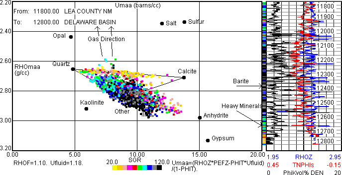
The above RHOmaa-Umaa plot suggests the Wolfcamp consists of quartz, calcite and clay minerals. The plot also suggests the density, neutron and PEFZ logs are well calibrated.
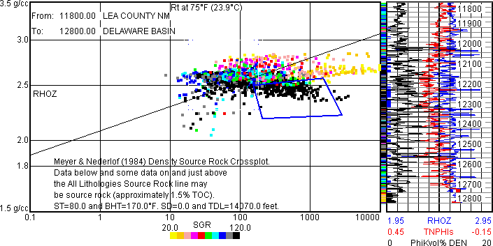
The above Meyer and Nederlof density source rock plot suggests the highest TOC Wolfcamp rock is within the blue polygon at depths with blue ticks to the left of the log plot.
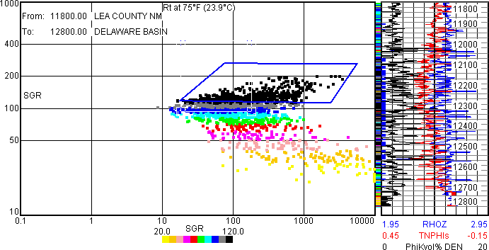
Increasing GR and increasing resistivity (Rt) as within the blue polygon above can aid in source rock identification.
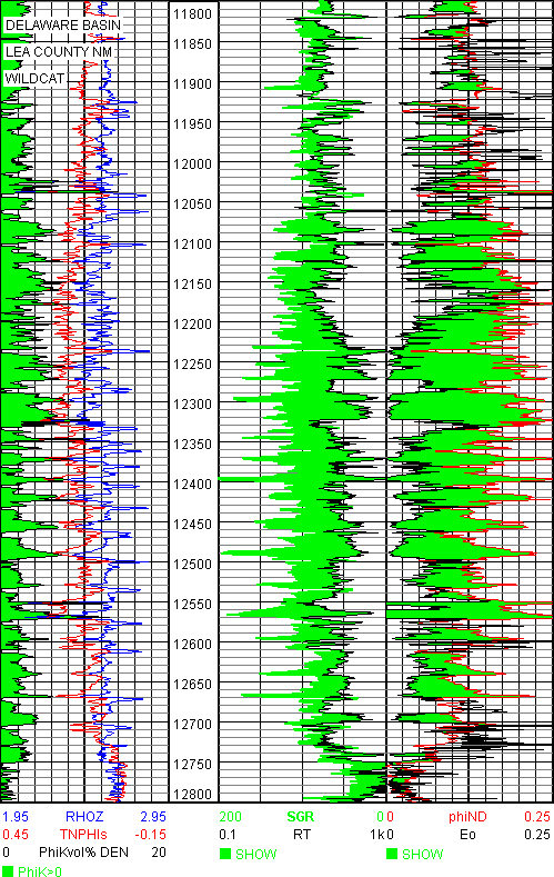
Separation between Eo and density-neutron porosity (phiND) appears to identify the Wolfcamp "sweetspot". Eo is based on "Pore Systems: Conductivity and Permeability", David C. Herrick, April 22, 2014, DWLS spring workshop. Eo=Co/(Cw*PHIT). Even though Rw was just estimated to be 0.50 and m=2.0.
2: NIOBRARA
JLog Calculated Curves such as Passey DlogR and Haecker TOCDEN can be used as a simple and rapid reconnaissance means to identify potential unconventional tight oil pay.
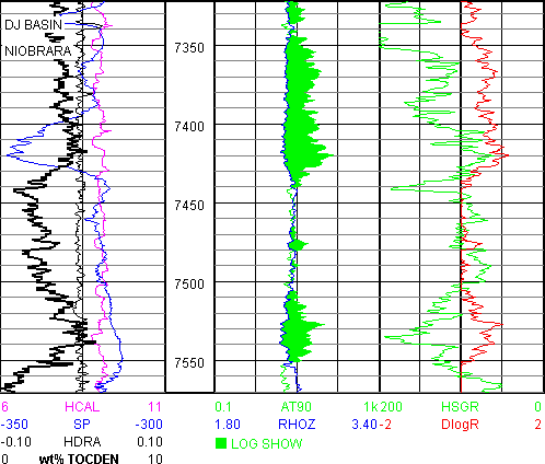
Two carbonate tight oil Niobrara models follow. Neither is "correct" but both identify prospective pay. The first is based on Density-Neutron crossplot porosity PHIE instead of PHIT in the Archie Sw model. The second uses Density porosity corrected for organic matter (kerogen) based on Haecker TOCDEN and pyrite.
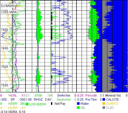
Note how the bulk density and resistivity identify pay in Track 2 above.
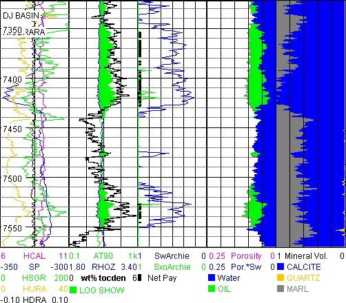
Passey TOCwt% is called TOCwt% DLR in version 9 onwards to diffentiate between a log curve TOC name or wt% TOCDEN. Niobrara LOM for TOCDLR and TOCDEN parameters are from paper Q, SPWLA 57th Annual Logging Symposium, 2016, Haecker, Carvajal & White. Thanks to Adam Haecker, personal correspondence, some of these parameters can be found in the Source & Tight Oil Manual shipped with JLog.
The Density-Neutron porosity model arrives at 31,400,000 BBL and the Density porosity corrected for organic matter and pyrite model yields 22,500,000 BBL OIL in place per section (640 acres) and both identify the most likely productive zones. These BBL OIL answers should only be taken as indicators because the Niobrara is not an "Archie" rock.
The following SW-POROSITY plots can be used to compare the two Niobrara models above. The most likely productive rock within the blue polygon is flagged at the left edge of the log plot. The first plot uses Sw below 0.4 and the second uses PHI*Sw (BVW) below 0.04 to flag data within the blue polygon.
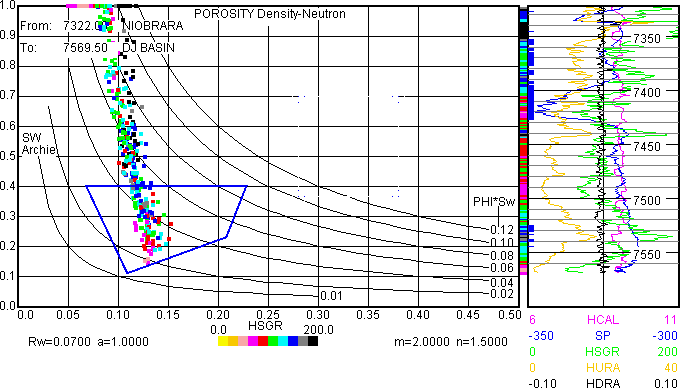
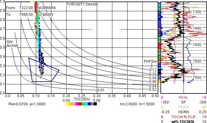
There is no known "Unconventional Archie" rock wireline log analysis model. An approach that correlates a consistent porosity and Sw model (even though wrong) and TOCDLR and TOCDEN to production is suggested as we try to better understand these reservoirs.
3: MOWRY
Next follows the Modica and Lapierre model that estimates kerogen porosity (PhiK) under certain conditions. PhiK is explained in Calculated Curves.pdf and a detailed example can be found in the Source & Tight Oil Manual.
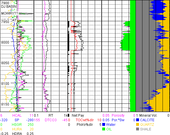
Note the increased radioactivity (HSGR and HURA-uranium) opposite the increased PhiK porosity around 8000 feet. 5,570,00 BBL OIL/640 acres are estimated from 7950 to 8025 feet.
B: Gas Shale
A Niobrara Gas Shale evaluation follows.

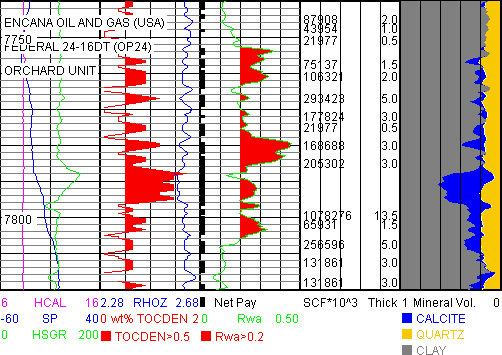
The Evaluation plot above finds gas in place computed with the Gas Shale model using the 3-Mineral PEF model for lithology. Rwa and TOCDEN aid in identifying hydrocarbons and organic matter in shale.
C: Clastic Reservoir
The three Eval plots that follow use different Evaluation models in a conventional quartz sand reservoir. These three plots are from SAND.TXT shipped with JLog.
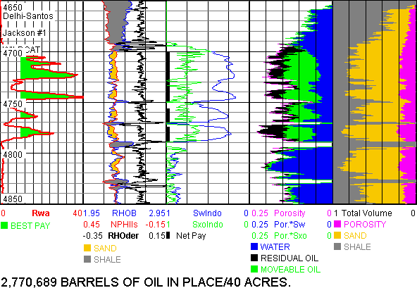
The Eval plot above uses Vshale from the GR that works well here but not in all reservoirs. Vclay is called Vshale for Indonesian Sw from version 10 onward.

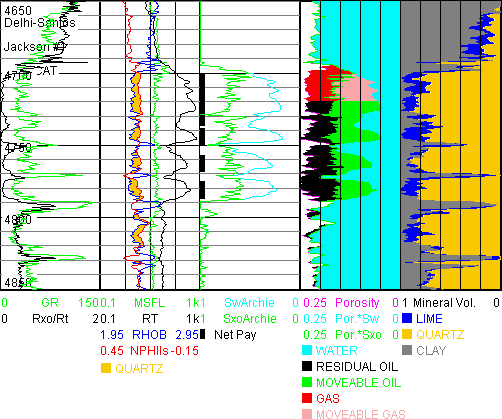
The Eval plot above uses the 3-Mineral PEF model for lithology while the plot that follows uses the 3-Mineral Sonic model with a hypothetical gas-oil contact set at 4720 feet.

D: Carbonate Reservoir
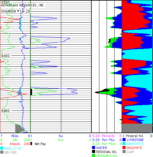
The Eval plot above (from CARB.LAS shipped with JLog) uses the 3-Mineral PEF model for two carbonates plus anhydrite and an override for Clay. Overrides can extend the model by use of filters calling various porosity models. This is useful for extending limited data sets.

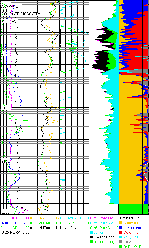
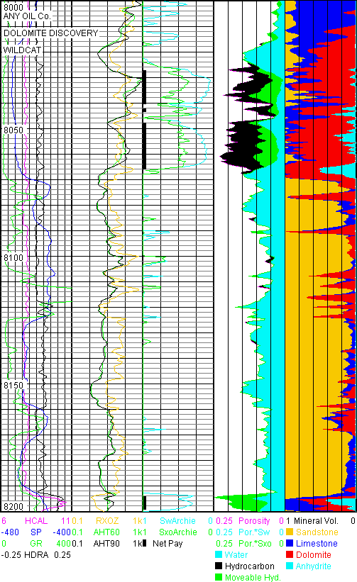
The Eval plot above (from DOLO.LAS shipped with JLog) utilizes the 5-Mineral (carbonate + clay) model from SPE 12597, McGinley & McKnight, 1984 (M&M). This model differentiates radioactive dolomite from clay or shale and uses the sonic to estimate clay or shale content. Very useful when dealing with radioactive carbonates that can be confused with shale. See JLog Workflow Example for 5 Minerals that follows near the end of this document.
E: Source Rock

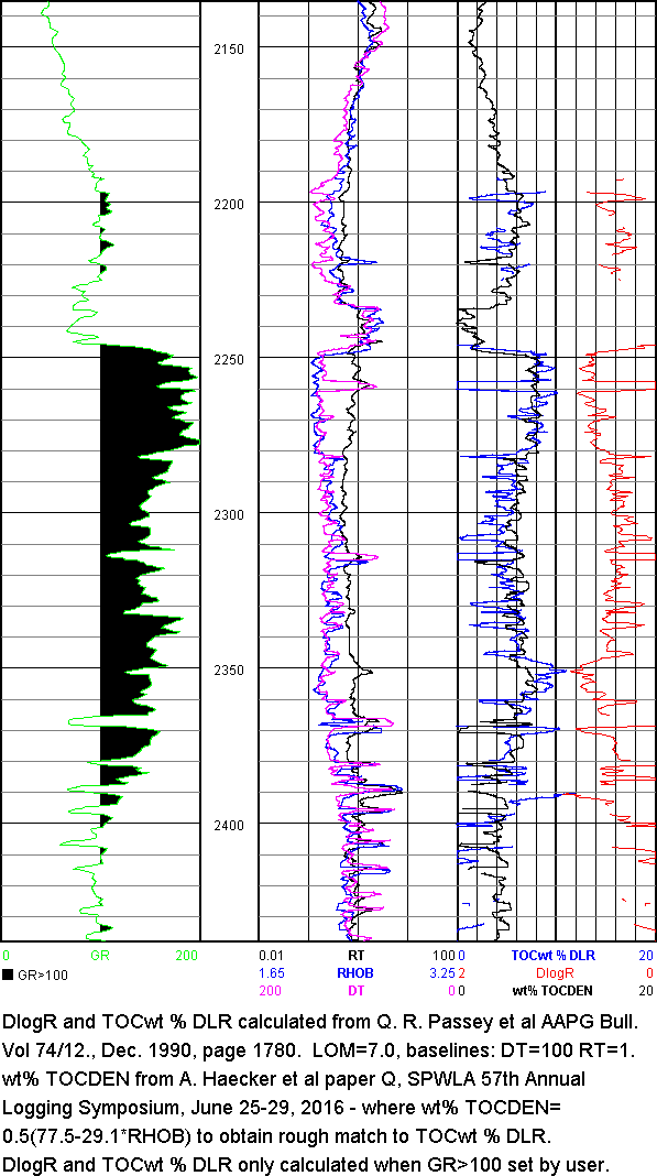
The 1/1000 log plot above (from SourceRock.JLG shipped with JLog) uses both the Passey delta log R (TOCwt % DLR) and Haecker density (wt% TOCDEN) methods to estimate TOC weight %. TOC volume % may also be computed from either. TOC estimation is important since it is now recognized that shale gas and tight oil are associated with TOC and that organic matter porosity can be an oil reservoir. When lab (LECO or Rock-Eval) TOC and Rock-Eval S1 and S2 are available S1 and S2 may be computed from a relationship with TOC. Then S1 and S2 barrels of oil can be computed.
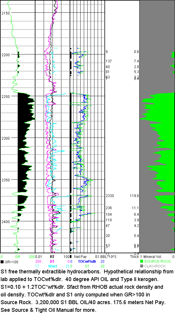
The Eval plot above uses a relationship (hypothetical here) between lab based Rock-Eval S1 and TOC (wt %) applied to Passey delta log R TOC (TOCwt%dlr) to estimate S1 free thermally extractible barrels of oil if within the oil window. This can be free oil residing in kerogen porosity or any other pore space and may represent free oil reserves in tight oil rocks.
Another relationship between lab based Rock-Eval S2 and TOC (wt %) applied to TOCwt%dlr can be used to estimate present day remaining source rock potential in barrels of oil.
Sfact in track 2 is the conversion factor based on rock bulk density and oil gravity applied to S1 to obtain BBL OIL. Some use a constant 21.89 for Sfact while JLog calculates Sfact at each depth based on bulk density log and input API oil gravity. A constant bulk density value can be input if needed.

The Eval plot above uses wt% TOCDEN to estimate S1 BBL OIL. It is recognized that an important part of S1 can be lost between core or cuttings and the laboratory and that some S1 may be in the S2 peak - so S1 is likely to be low.
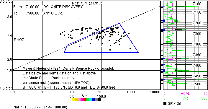
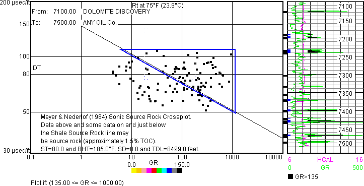
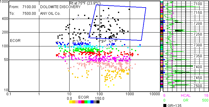
The following are three quick Source Rock plots to identify source rock. Likely source rock data within the blue user-drawn polygon is highlighted at the left edge of the log plot with blue ticks.
The first two plots that follow are based on work by Meyer and Nederlof (1984).


Generally, marine source rock has increasing resistivity associated with increasing GR as seen below.

More mature source rock generally has increased resistivity, up to a point.
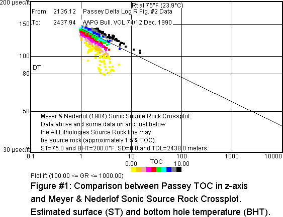
The plot above shows how the Passey delta log R TOC method compares to that of Meyer & Nederlof.
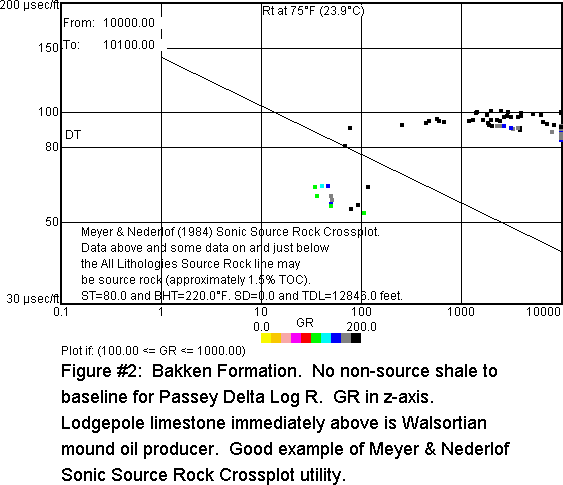
Meyer & Nederlof (M&N) has the ability to quickly identify source rock when it is not possible to find a shale baseline needed for Passey delta log R method. But M&N does not estimate TOC.
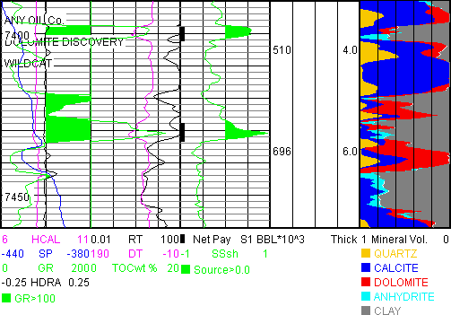
The plot above shows good agreement between Passey delta log R TOCwt% and M&N methods for source rock identification. M&N (Source SSsh>0.0) supports the Passey TOC shale baseline resistivity and sonic value selections. The 5-mineral M&M model is in the far right track.
1,206,000 BBL S1 oil/640 acres are present over 10 feet, based on reasonable hypothetical values. See the Source & Tight Oil Manual for workflow and variables selection.
Information
JLog is designed for those who do log analysis from time to time on unconventional reservoirs and conventional reservoirs with one or many zones that have all the same characteristics such as Rw, Rmf, GRclean and so on.
JLog is coded in the Java® programming language so it has the potential to run on different operating systems equipped with the appropriate Java Runtime Environment (JRE) and USB port security key (aka dongle). A JRE for Windows is shipped with JLog and may be installed if not already installed (most Windows machines already have a JRE). Download instructions are included if Mac does not have a JRE.
JLog users need access to an e-mail account should they need free support.
JLog imports LAS and TEXT (ASCII) files of unlimited length and exports answers in LAS and TEXT files. JLog handles depth in both meters and feet and up to 63 log curves and many additional Calculated Curves. Graphics can be saved in four graphic file formats.
JLog calculates and plots the following Calculated Curves if the appropriate logs are present: Khoyle, phiS, phiND, RHOmaa, Tmaa, Umaa, Rwa, Rmfa, PHIT, PHIE, Vclay, Sw, Sxo, BVW, BVH, Ktimur, % VRE, ADSscf, DESscf, PoiRat, ShearM, YoungM, MHSG, MHS, Ratio, Ro, FOIL, SwFOIL, BulkM, TOCDLR, DlogR, TOCvol, S1, S2, Sfact, S1/TOC, S2/TOC, S1+S2, PI, S3, OI, BRIT, pBRIT, BRITpe, sBRIT, BRITdt, Rxo/Rt, AcImp, RefCf, Vp/Vs, Source, ShQual, Eo, iTOC, iTOCvol, PhiK, TOCDEN and DIFF (first derivative). See JLog Calculated Curves.pdf (shipped with JLog) for explanations and descriptions of the Calculated Curves.
- No environmental corrections are applied. However RT is estimated from Schlumberger Chart Rint-9 when Rxo, LLS and LLD or equivalent curves are available. This computation is made for all logging contractors so the resulting RT may not be absolutely correct for all Rxo, LLS and LLD combinations but it will generally be a better RT estimate than LLD.
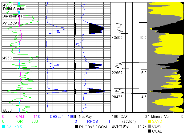
- JLog is shipped with a sandstone Text file (SAND.TXT), a carbonate LAS file (CARB.LAS) and a dolomite LAS file (DOLO.LAS). SAND.TXT includes productive shaly oil sands (4,700-4,800 feet) and coals (4,900-5,000 feet). DOLO.LAS contains dolomite pay and source rock. These files can be used to self-train on JLog. Thanks to Delhi Santos and Wiltshire Geological Services of Adelaide, South Australia, for the SAND.TXT well logs. Thanks to Advantage Resources, Inc. of Denver, Colorado for the CARB.LAS well logs. Thanks to the companies that posted log data on the Colorado Oil and Gas Conservation website. SourceRock.JLG and NIOBRARA.JLG can be used to test the Source Rock and Tight Oil models respectively (both also shipped).
- Appropriate density-neutron crossplot porosity estimates are available for Neutron Logs including: APLC, CNC, CNCF, NPHI, NPOR, NPRL, NPRS, NPRD, SNP and TNPH. The porosity estimate is not just a simple average of density and neutron porosity values.
- A wide variety of lithology crossplots with vendor and log specific overlays are available to check log quality and identify lithology. JLog includes the following lithology crossplots if the logs are available: Density-Neutron, Density-PEF, RHOmaa-Umaa, MN, MID (RHOmaa-Tmaa), Tmaa-Umaa, Sonic-Neutron and Density-Sonic. The RHOmaa-Umaa plot is used to select end points for the 3-Mineral PEF model while the MID plot is used to pick end points for the 3-Mineral Sonic model (mineral-3 from both can be Vclay). The RHOmaa-GR plot is used to pick Vclay clean and clay endpoints and test for clayey sand gas effects. Source Rock plots aid in rapid source rock identification. Interactive Pickett and Rxo-RT plots quickly estimate m, Rw, Rmf, Sxo and Sw. Resulting Rw and m are saved for the evaluation and can be changed later. The Density-GR plot is used to select coal, rock and clay endpoints. PHID-GR and PHID-Vclay plots aid in estimating clean sand porosity for the Thomas-Stieber laminated sand model. Up to 4 filters can be applied to all crossplots and histograms to view critical data patterns.
- Density, sonic and GR Source Rock crossplots are available that help in source rock identification.
- Users can plot Track 1 logs at various depth scales to the right of the crossplots with Z-axis colors plotted between the crossplot and the logs so users can can match crossplot data to depth and the logs.
- Users can select a Lithology, Source Rock, Pickett, Rxo-RT and User data group wiithin a user-defined blue polygon. A blue tick will be placed at the left edged of the log plot for each data point that lies within the polygon. This aids in correlating polygon data with log response and depth.
- Users can shade above/below and between log curves with 10 colors and add a short legend to emphasize important points.
- Appropriate Vclay (up to 10), Porosity, shaly sand, laminated sand (Thomas-Stieber), sand-silt-clay, carbonate, two 3-mineral lithology models and 7 Sw models allow the user to quickly estimate hydrocarbons in place. Coal Bed Methane Gas analysis uses the Clay Rock Coal model. Gas Shale analysis and Pulse Neutron models are also available. The Source Rock model estimates source rock hydrocarbon values.
- Answer curves such as porosity, Vclay, Sw and mineral volumes are calculated on the fly and are available for viewing and export in LAS and TXT files. All the Calculated Curves may be included in the saved LAS or TXT file.
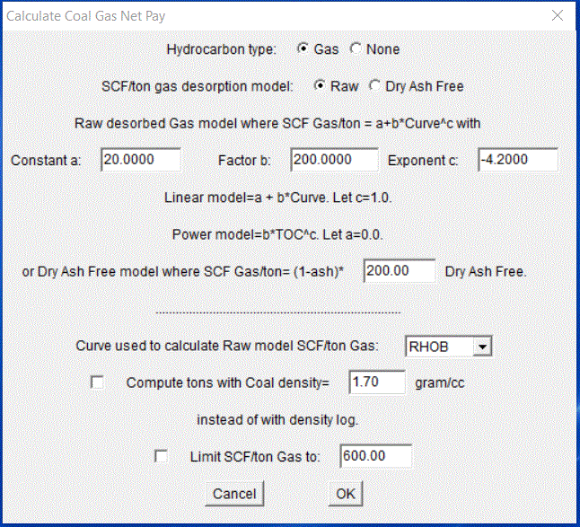
- Calculated Curves such as Khoyle (carbonate permeability indicator), Rxo/RT, Rwa and Rmfa assist in identifying potential reservoirs and hydrocarbons. ADSscf and DESscf calculations in the form of a+b*Curve^c may be plotted. Coal Bed Methane Adsorption and Desorption is often related to the density log with a function or transform of this sort. Mechanical rock properties Calculated Curves are available if shear and compressional sonic along with density are present.
PoiRat- Poisson's Ratio. need DTc and DTsh.
ShearM-Shear Modulus. need DTsh and density.
MHSG-minimum horizontal stress gradient. need DTc and DTsh. user inputs Biot's poroelastic constant and reservoir, overburden and tectonic pressure gradients.

- The plot above with Calculated Curves Rxo/Rt in Track 1 and Rwa in Track 3 identify pay while AcImp and RefCf in Track 3 can aid in seismic understanding.
- Calculated Source Rock curves include TOCDLR, DlogR, S1, S2, Sfact, S1/TOC, S1+S2, PI, S3, OI, Source, ShQual, iTOC, iTOCvol, TOCDEN and PhiK. An explanation of these Calculated Curves and the Source Rock Eval Mineral Model is found in the separate Source & Tight Oil Manual folder. Open SourceRock.html inside with a web browser to proceed with these models. Also see JLog Calculated Curves.pdf
- Net pay based on user determined cutoffs is flagged in graphics and computed in text tables for perforation selection and export.
- Hydrocarbon reserves are estimated from the summation of level by level calculations.
- The best way to check out JLog is to scroll through the JLog User Instructions that follow. A number of features will be demonstrated but not all. Working down each menu is the best way to check out JLog capabilities. You will see various plots, models and graphics along with Windows and Mac interfaces.
- It is not necessary to demonstrate every feature here in the JLog User Manual since JLog users are intelligent and creative. Source & Tight Oil and FOIL User Manuals are also shipped with JLog.
- JLog features and output can be combined with other software to solve problems and to convey ideas to others.
JLog User Instructions
Here are a number of steps one can take to perform an evaluation. There are many JLog ways to estimate lithology, source rock, in-place oil and gas and identify unconventional reservoirs. Working through all the menu items and experimenting will be time well spent.
Section I: File Menu
Here data is imported, graphics saved as GIF, BMP, JPG and PNG file types for export to other applications for display, reports and printing. Data and answers can be saved as TEXT and LAS files for export to other applications.
With the View button of Import... of the File menu one should always open TXT and LAS files to view the curve names and LAS header information such as curve names and units. Correctly structured LAS files should explain the curve names and units in the ~Curve Information block. All curves should be imported in order to enable the appropriate JLog features.
One can also open the TXT or LAS file with a word processor and view and print the header.
With the View button of Import... of the File menu open SAND.TXT and you will see the following logs in a spreadsheet format of columns and rows. Never use Open of the File menu to open LAS or TXT files. The first row contains the curve names:
Depth MSFL LLS LLD RHOB NPHI GR PEF DT SP CALI
The data appears in a spreadsheet arrangement below each curve name.
It is generally not a good idea to change the curve names. An exception would be an input TXT or LAS file that has density only in the form of density porosity such as DPHI. You could change the DPHI name to RHOB prior to import and then convert to bulk density when importing by advising JLog of the RHOF and RHOG values used to compute DPHI. If possible, always ask for the bulk density itself in the LAS file - JLog can compute density porosity from it later on.
If one wanted to read log values from hard copy logs they could enter values by hand and construct a spreadsheet similar to SAND.TXT and save it as a tab delimited TEXT file. Each column of data must be filled in. If data is bad or missing just enter the null value of -999.250. It is not necessary to enter the log data at uniform depth increments but it is better to do so. The depth increment could be larger for a thicker pay zone than for a thin one.
NPHI is in percent limestone porosity units here but JLog wants the units in decimal. You will have a chance to convert from percent to decimal when importing the SAND.TXT data. If NPHI is in sand or dolomite porosity units JLog will convert them to limestone.
It may be useful to open the Text (TXT) or LAS file to be imported with a word processor or text editor so you can see the curve names and check the actual data.
Choose and push "TXT" button as File type of Import... of the File menu.
Then push the Import button and find and open SAND.TXT.

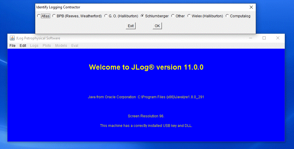
The first dialog asks for the Logging Contractor which is Schlumberger. The presentation shown above is the same as in previous JLog versions. There are no dramatic interface changes from version to version. Choose and push the "Schlumberger" button. It is important to correctly identify the Logging Contractor so that the correct lithology overlays, neutron matrix conversions and density-neutron porosity models will be used. The Atlas button refers also to Baker Atlas and Baker Hughes. The BPB (Reeves, Weatherford) button may also apply to some Precision logs. Check with your logging contractor. Note the last line of text in the blue JLog window above that indicates the USB key is in place along with the Sxjdk.dll DLL file in the JLog folder. Above that you will find the location of the Java Runtime Environment (JRE) in C:\Program Files on Windows 10 PC.
Note the "Logs in the TXT File to be Imported" in the bottom window that follows. Click OK. Then the dialog asking for SP and Caliper curve names will follow along with others. To abort the import process click Exit.

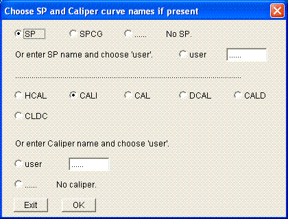

Next you will be asked for the SP and Caliper names. Look at the bottom window entitled "Logs in TXT File to be Imported" to see what logs are present. There is an SP called SP and there is a Caliper called CALI so push the appropriate buttons which are "SP" and "CALI". JLog will automatically push the correct button for some commonly used curves. Always check because if the correct button is not pushed the default may not match the curves to be imported. If the Caliper was named CALX you would type in CALX and choose and push the "user" button for Caliper. Be sure to remove the .. since CALX.. will not be recognized - it must be just CALX and note that the names are case sensitive so you cannot enter calx for a CALX name and have calx recognized. If no Caliper curve was present you would choose and push the "No caliper." button. Remember, you need to always check the logs in the bottom window to be sure the appropriate curves are imported. Click OK.
Next you are asked to Select GR if present. There is a GR so choose and push the "GR ...... ...... ...... ......" button and click OK.
Next you are asked to select micro log and Rxo curves if present. There is a MSFL so choose and push the "...... ...... MSFL" button. A pair of six dots ...... ...... denote the absence of micro log curves. Click OK.
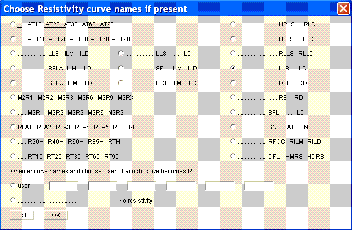

Select Resistivity curve names if present. LLS and LLD are present so choose and push the "...... ...... ...... ...... LLS LLD" button. Click OK. Note the deepest resistivity curve placed in the far right slot will be taken as RT except for laterolog curves equivalent to LLS and LLD (HRLS HRLD through RS RD in the dialog box above) where RT will be estimated as mentioned earlier. RT will also be computed from hand-entered laterologs that begin with LLS and LLD such as LLSEC and LLDEC with version 9 onwards. Many of the common resistivity combinations are found in the buttons above. Note how the resistivity curves with shallowest depth of investigation are on the left with the deepest depth of investigation curve on the right. Suppose the dual induction resistivity curves are RLL3, RILM and RILD and are not found in the button array above. In this case RILD would be typed in the far right user slot #6 and becomes RT. RILM is typed in slot #5 just to the left of RILD and RLL3 is typed in to the left of RILM in slot #4. The first three user slots would each remain empty with ...... . Be sure to push the "user" button so the three new curve names will be recognized and imported by JLog. Then Click OK.
Please note that all six ...... have to be removed when typing in a user curve name such as RLL3, RILM and RILD. Do not leave any dangling . when typing user curve names. For example, typing RILD.. will not be recognized as an incoming RILD resistivity. RILD must be typed for RILD induction and so on.
Select Density and PEF curve names if present. Both RHOB and PEF are present so choose and push the "RHOB ...... PEF" button. Click OK. Here is the place to import RHOB, RHOZ, ZDEN, DEN and other bulk density log values. If calculated density porosity curves such as DPLS, DPHI, DPOR and PHID are also present they may be entered by hand and imported later under Add more curves..?
If a calculated Density porosity called DPOR is present, without the actual bulk density value, then type in DPOR in the first slot to right of the user button like this: DPOR do not leave any . after DPOR since DPOR.. will not be recognized. If there is no bulk density correction or PE curve then the next two slots will remain ...... don't forget to push the "user" button after filling in the density porosity curve name.
See Tip #20 of JLog tips.doc when there is only a density porosity curve available. If you are digitizing logs always try to get the actual bulk density log digitized if possible instead of the density porosity.
Select Neutron curve names if present. There can be up to 3 neutron curves in some (Schlumberger Platform Express) data files. After all the neutrons are imported the user can select any one to work with when doing the log analysis. It is important that the actual logging contractor curve name be used. Do not use a third party made up name. For example if importing a set of logs with ZDEN density and PNLS neutron you need to edit the incoming file so the actual Atlas neutron curve name such as CNC is used. Otherwise you can import the PNLS neutron and Edit it with Add New Curve Names... of the Edit menu. Other Contractor neutron logs are treated as Schlumberger NPHI. Here we only have NPHI so we choose and push the "...... ...... NPHI" button. Click OK.
Select Sonic curve name if present. We have DT so choose and push the "DT ...... ...... ...... ......" button. JLog can handle and import up to two compressional and three shear sonic curves if present. Click OK.
Add more curves? If there were more curves we can add them or we can also add a curve one more time but since there are none we choose and push the "Do not add any more curves" button. If there were more curves to be added choose the "Add up to 33 more curves" button and type in the new curve names that appear in the bottom window. If we wanted RHOB duplicated we would type in the RHOB name and a 2 would be appended to the name yielding RHOB2 in the JLog file. Remember the curve names are case sensitive.
Identify Density units in incoming file. When we inspected the SAND.TXT file we saw RHOB values expressed as 2.32, 2.45 and so on. These units are gram/cc so the "G/CC" button is pushed. If the values were expressed as 2320 the units would be K/M3, if 20.0 then units are Porosity Percent and 0.20 Porosity Decimal. In the last 2 cases we would be asked for the RHOF and RHOG values used to compute the porosity because we want our density in grams/cc. We would also want to change the density curve name from DPHI to RHOB in one of two ways. First by changing DPHI to RHOB in the ~CURVE block of the LAS file header before import or after import with Add New Curve Names... of the Edit menu. See Tip #20 of JLog tips.doc for more.
Identify Sonic units in incoming file. When we inspected the SAND.TXT file we saw DT values expressed as 82.4 and so on. These units are in microseconds/foot so the "US/F" button is pushed. Other units might be microseconds/meter (US/M) or milliseconds/meter (MS/M).
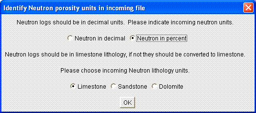
Identify Neutron units in incoming file. When we inspected the SAND.TXT file we saw NPHI values expressed as 30.00 and so on. These units are in limestone percent. Logging contractors do not always identify neutron porosity lithology units in their data files so check the hard copy logs for neutron lithology. Here "Neutron in percent" and "Limestone" buttons are pushed.

SAND.TXT neutron porosity units are in percent so the "Neutron in percent" button is pushed by the user. JLog will push the correct button for you in correctly constructed LAS files.
Always ask the logging contractor to include the density in gram/cc and neutron porosity in limestone decimal porosity units in the LAS file regardless of the lithology and the scales used on the hard copy logs. Also request near and far neutron counts in the LAS file. Additionally check that digitized neutron porosity units are correctly stated in the LAS file. This also holds true for density when units are not in g/cc.
The following information would come from the hard copy logs. If we were importing a LAS file the information might be present in the LAS file. But not necessarily. It is always a good idea to have the digital images or hard copy logs of at least the log headers available. Default values that follow are appropriate for Jackson #1 data in SAND.TXT. This information must be changed for other wells.
Company Name: Delhi-Santos. Well Name: Jackson #1. Field Name: Wildcat
Click OK.
More Well Information: STATE: Queensland. COUNTRY: Australia.
Click OK.
Mud, filtrate and mud cake Resistivities:
First choose and push the "Fahrenheit" and "Other" buttons.
Rm: 1.080 at 86.0 Fahrenheit.
Rmf: 0.752 at 71.6 Fahrenheit.
Rmc: 1.308 at 66.2 Fahrenheit.
Note: the engineer actually measured the various mud resistivity and temperature values.
Bit Size and zoned Bit Size:
Bit Size: 8.50.
If there are several Bit Sizes you may enter them along with the appropriate interval.
Depths, Temperatures, Fluids and Units:
Select feet and lb/gallon. Fahrenheit is already selected.
Depths Surface: 0.00. Bottom Logger: 5727. Depth Reference Elevation (usually KB): 396.00.
Temperatures Surface: 80.00. Bottom Hole: 217.
Fluid Density: RHOF (G/CC): 1.0.
Drill Fluid Density: 9.70 lb/gallon.
The default JLog file name is the Well Name.
File name: Jackson #1.JLG
Click OK or SAVE or whatever is appropriate for your operating system when you name a new file. Be sure the .JLG upercase file extension is present so the file can be identified by JLog later on. Windows users need to have file extensions turned on so the .JLG can be seen - important if making your own file name.
Once the file is converted you will be notified. Open the resulting JLog (.JLG) file with Open... of the File menu to start the log analysis. Never open a TXT or LAS file with Open of the File menu - it is just for JLG files.
Save As... menu item. The most recent graphic plot can be saved in GIF, BMP, JPG or PNG format. That graphic file can be opened with a graphics application and printed or imported by another application for presentation purposes.
Logs, Calculated Curves and Eval answers may be saved in LAS and TXT file formats.
Section II: Edit Menu
Here the user can add well information, add new curve names, compute Rw and add plot legends.
With Open... of the File menu find Jackson #1.JLG and open it.
Work down the first 4 menu items of the Edit menu and you will see the well data that was entered when making the JLog file. That information is saved in the Jackson #1.JLG JLog file. It is a good idea to check this data and correct it if necessary.
Add New Curve Names... allows the user to change the curve names. You might want to do this after importing a meaningless pseudo curve name. For example if you imported a set of Atlas logs with a PNLS neutron you can change PNLS to CNC which is a proper Atlas curve name. JLog would not recognize PNLS but will recognize CNC as far as crossplot overlays and crossplot porosity is concerned. The JLog file has to be closed to use this feature.
The Rw submenu contains routines for calculating fluid resistivity (Rw or Rmf) at reservoir depth and Sigma fluid from measured Fluid Resistivity and temperature or Salinity (see Tip #33 of JLog tips.doc), Rw from the SP and percent formation water from wireline test samples or DST samples. Rw estimation from SP and salinity data is one of the first things done in a log evaluation.
The Annotations submenu contains Well Information... and allows the user to enter text for Plot Legend... . Text Font and Size can be changed in the File menu.
The Conversions submenu contains Tmax to Ro... and Ro to Kerogen Density... conversions. Ro is Vitrinite Reflectance %.
Section III: Logs Menu
Here log data is viewed, presentations for log plots are set and logs are plotted.
Next we should look at the data with View Log Values... of the Logs menu to check the log data.
Set From at 4500 and To at 4520. Click OK. After a brief wait the log data will appear in a table. View Log Values... can handle 1000 levels of text - it is designed to check that the log data is correctly imported.
Notice the RT values computed from MSFL LLS LLD in column 8. These RT values will be used for Pickett plots and the evaluation unless the user selects another curve for resistivity. Note NPHIls in column 12. ls has been appended to denote limestone lithology. We (JLog) need the neutron in limestone decimal porosity units for cross plotting and the computation of density-neutron crossplot porosity. That is one reason why it is useful to have the neutron in limestone porosity in the LAS file. That saves JLog from converting the neutron to limestone porosity if it is only in sandstone or dolomite porosity.
In the upper split window you will see some well information.
The Setup Logs Tracks... menu item has options for log presentations. Click OK when finished. Experiment here to see which presentation best fits your log data, computer screen width and print paper size if printing saved graphics later on.
Plot Which Logs?... allows the user to decide which logs to plot by checking the checkbox, selcting the Color, Weight (trace width 1-3), Track and Left and Right Scale. If Logarithmic is checked the log will always plot in Track 2. Logarithmic scale is not appropriate for logs that contain values at or below zero. You may need to scroll to reach the OK button at the bottom of the dialog box. The "Backups" checkbox gives the option to plot the logs and Calculated Curves without backup (wraped) curves. This can tidy up a messy plot that has a lot of backup curve activity. Click OK when finished.
With 1/500... of Plot Logs plot from 4700-4850. Type 4700 after From: and 4850 after To: and Click OK when finished. This is the pay zone and the water zone just below. The oil/water contact is somewhere within the shale starting at 4790 feet. Rw is around 1.0 to 1.5 ohm.m and Rmf is about 0.450 at reservoir temperature based on RT and Rxo Pickett plots that can be made later.
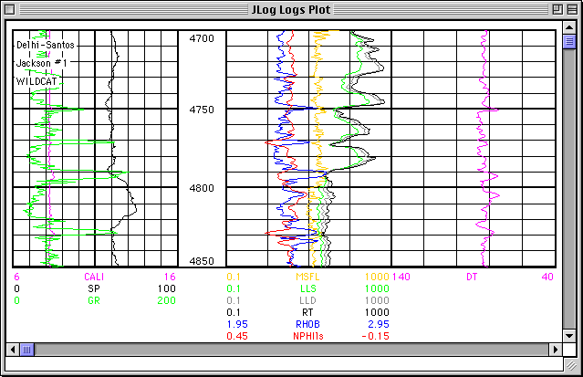
This is how the default setting of the logs would look if the user makes no changes to setup, presentation and which logs to plot.
Go back to Shade Between... menu item.
Check the first Shade checkbox on the top row. Select "red" Color in the first row opposite the checked box.
Between Left Log column, top row, select "LLS" and under and Right Log column, top row, select "LLD" from the dropdown menus.
Under Shade Legend, top row, type in "PERMEABLE".
We are shading between LLS and LLD and coloring it red thus suggesting the resistivity separation is due to permeability. Click OK.
With 1/500... of Plot Logs of the Logs menu plot from 4700-4850. Click OK when finished. Notice the red color between the LLS and LLD in Track 2 below and the PERMEABLE legend after the small red box.
Go to Shade Left or Right... menu item.
Check the first Shade checkbox, first row. Select orange Color in the first row opposite the checked box. Click "To Left of" button. Select "GR" from the dropdown menu. Under Value enter "50". Under Legend type "CLEAN SAND". Click OK.
With 1/500... of Plot Logs plot from 4700-4850. Click OK when finished. Notice the orange color below GR values of 50 and the CLEAN SAND legend after the small orange box under Track 1 below.
Results can be seen below in the 4700-4850 foot plot that follows.
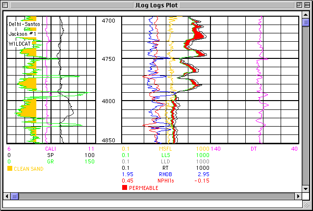
These two shading techniques illustrate a way to convey your ideas to others prior to log analysis. You need to know something about the rocks and the log response to the rocks to make this meaningful. Note GR Right Scale is now 150 and CALI Right Scale is 11. These scale changes assist in the presentation. Since there is very little movement on DT perhaps a 100-50 scale would be more appropriate.
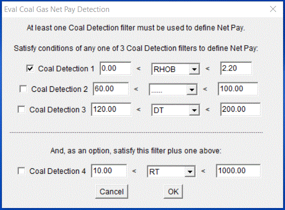
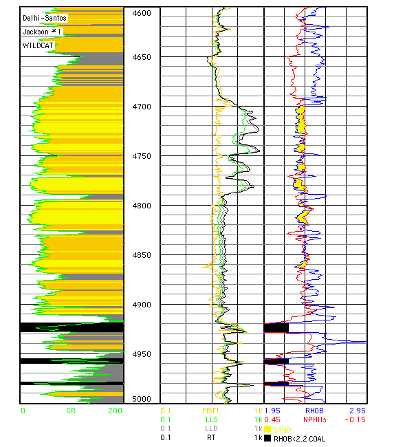
Shade Stratigraphy... can be used to show sand, silt and clay intervals by shading a single curve that relates to stratigraphy and lithology. In the example that follows "Stratigraphy Shade" is checked and GR is selected from the dropdown menu. Yellow<35 and Orange<70 are entered. The "Shade Coal black." checkbox is checked and "Coal Detection 1" checkbox is checked and is defined by 0.0 < RHOB < 2.20. Same as set under Models/Eval Mineral Models/Coal Detection... . Shade Between... has been used to shade yellow when RHOB is to the left of NPHIls caused by quartz (SAND) effect on the 2 logs run on a limestone compatible scale. Results are seen below.
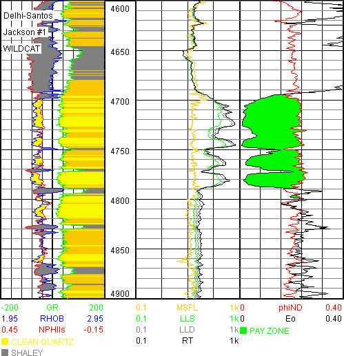
Comparison of Eo to phiND in the water zone above suggests both Archie porosity exponent m=2.0 and formation water resistivity Rw=1.5 are reasonable. Eo and phiND are Calculated Curves selected with Eval/Plot Which Calculated Curves?... .
Both m and Rw can be changed with Models menu Variables submenu and a, m, n, Rw and Rmf. Experiment with m and Rw changes to obtain a good match.
Set Margins... allows one to set margins that are useful for later print centering of graphic plots.
To save as a graphic file: select Save As... of the File menu and push the "GIF" button and name the file Jackson#1Logs.gif. This GIF file can be imported by other applications to be included in a report, printed or e-mailed.
Section IV: Plots Menu
Various lithology, source rock, Pickett, Rxo-RT and User (User Defined, Density-GR, PHID-GR, RHOmaa-GR, PHID-Vshale and Vshale-Rt) plots and Histograms are plotted implementing up to 4 filters. This helps lithology and source rock identification and estimates of m, Rw, Sw, Rmf and Sxo.
Z-axis... menu item allows the user to select measured depth (MDEPTH), a log such as GR or a Calculated Curve such as Rwa to be plotted in the Z-axis scaled in either color or numbers from a user determined Z-axis minimum to maximum value. GR in the Z-axis is often useful.
Caliper plotted in the Z-axis can identify data affected by hole washouts. Tfluid and RHOF may be needed for some plots and later for the evaluation.
When more than one neutron, compressional or shear sonic are present they may be selected with Which Neutron... , Which Compressional Sonic... and Which Shear Sonic... menu items.
The Litho & Source Rock submenu allows the user to plot a variety of lithology crossplots that aid in lithology and porosity estimation, source rock identification, selection of the correct evaluation model and determining if logs are affected by bad hole.
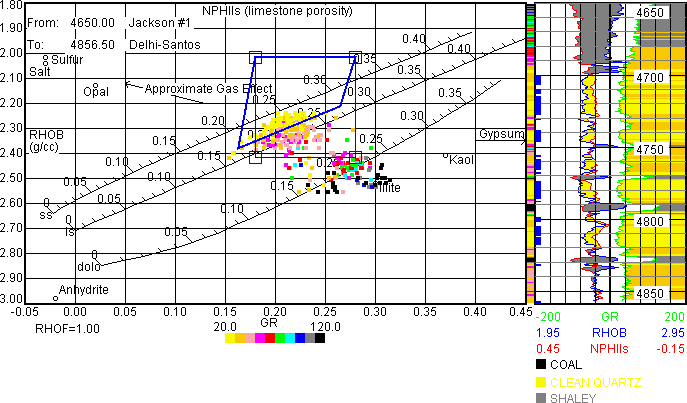
The Density-Neutron... is a key lithology plot for lithology estimation as well as porosity estimation. The plot above shows an increasing Z-axis GR as data moves away from the Sandstone (ss) line towards the Dolomite (dolo) and Illite clay point (shaly). Note the cluster of yellow data in the thick line blue polygon which suggests either calcareous or slightly shaly sand. The RHOmaa-Umaa... plot that follows will resolve this lithology question. The Density-Neutron plot can also be used to pick RHOB and NPHIls values for the Sand Silt Clay model as well as Sand and Silt grain density.
Data within the thick line blue polygon is flagged at the left edge of the 2 inch/100 ft (1/600)... log plot and that along with Z-axis colors plotted just to left of log plot aid in tying plot data to depth and log response. The thin line blue polygon represents the initial polygon before dragging 4 corner targets around to capture the user-required data cluster within the polygon.
Note the porosity scales for the 3 major lithologies: ss, ls and dolo. Total porosity (PHIT) is computed from equi-porosity lines running through the 3 porosity scales. Neutron logs are designed to correctly estimate porosity in 100% water saturated limestone. The sandstone and dolomite lines vary with the logging contractor, neutron detection method and tool type. This is why it is important to correctly identify the logging contractor and the proper neutron curve name during import.
The Trk 1 Logs with Plots and Highlight Data in Plots menu items have been selected and turned on and that allows one to plot Track one logs to the right of a Plot as seen in the Density-Neutron plot above and in several plots that follow.
The thin line blue square polygon with 4 small corner squares (targets) appears just after the plot is made. One then places the cursor in a target and drags the polygon around to capture data in the resulting heavy blue line polygon seen in the plot above.
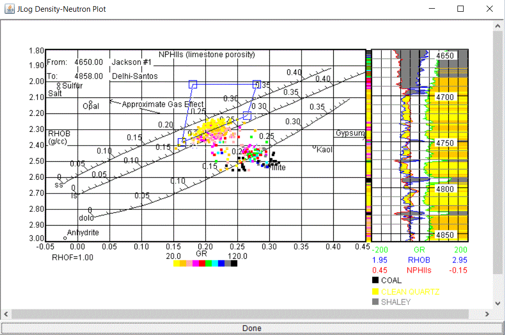
The plot above shows the 4 small targets that users drag, one by one, to place the blue 4 sided polygon around a data cluster. Once satisfied "Done" is pushed and the result may be seen 2 plots above with Plots/View Highlight Data and saved as a GIF file with File/Save As.../GIF.
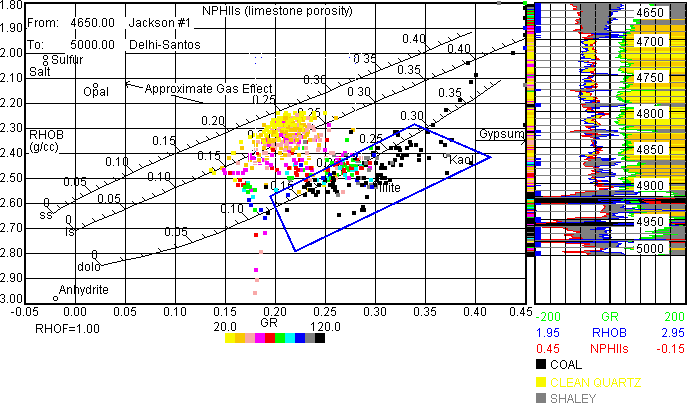
Here, above, the Density-Neutron plot covers more interval since the log plot depth scale has been changed from 2 inch to 1 inch/100 ft. Plotting stops when the Track 1 Logs with Plots run out of space to plot at the right hand side of the Plot. Clays and shales are falling within the heavy line blue polygon. Note the clays and shales may have higher bulk density (RHOB) than the very porous quartz sands higlighted in the previous Density-Neutron plot.
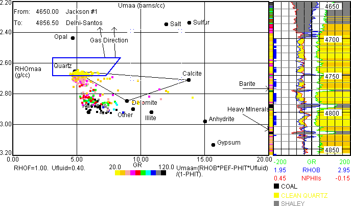
The RHOmaa-Umaa... plot above helps to resolve the lithology question in the RHOB-NPHIls plot. Clays and shales have higher Z-axis GR values. The 3 main lithologies are quartz, calcite (cement?) and clay or shale. Some heavy minerals (siderite?) are also present in thin beds. This plot will be used later to pick endpoints for 3 minerals in the 3-Mineral PEF models. Vclay (Vshale) can be mineral 3 for use in a shaly sand Sw model. Often a good idea, since GR can be a missleading clay (shale) indicator in some rocks.
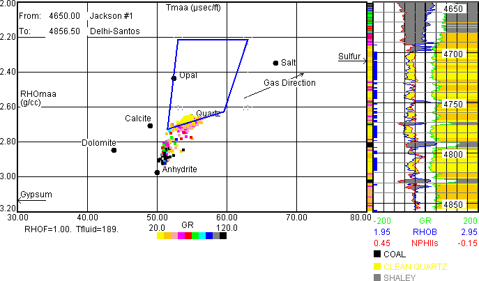
The MID... (RHOmaa-Tmaa) plot also helps identify lithology. The 3 main lithologies are quartz, calcite (cement?) and clay (shale) with higher Z-axis GR values. This plot was used to pick endpoints for 3 minerals in the 3-Mineral Sonic model with Vclay (Vshale) as mineral 3 shown earlier. Clay (shale) was picked at RHOmaa (RHOG)=2.90 and Tmaa=51. MID plot lithology identification is not always this good in unconventional reservoirs. No siderite effect is present.
All available lithology plots should be viewed in order to determine the likely lithology - only a few are shown here.
The Pickett submenu allows the plotting of Y-axis porosity against X-axis RT, Rxo or any other resistivity curve to estimate Rw, m and Rmf at reservoir conditions. Here we will use RT to obtain Rw in the water zone and an estimated Sw.
With Pickett Porosity... menu item select the porosity model to be used in the Pickett Plot. Try Density porosity here.
With Pickett Plot... menu item the user can make the Pickett Plot over a user defined interval such as 4700 to 4850 feet below.
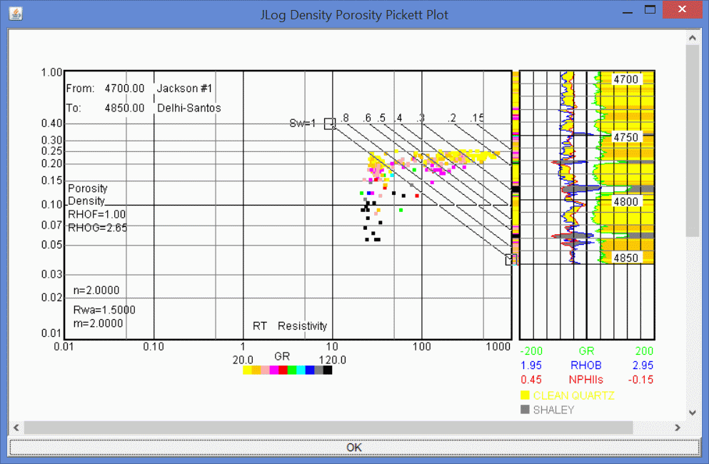
The user drags the small square targets, that appear at the end of the Sw=1 line, one by one, to change the fluid resistivity (Rwa here) and m (Archie porosity exponent). Generally one wants the Sw=1 (Sw=100%) line to fall on the lower resistivity, clean data pattern. Rwa and m are re-calculated as the Sw=1 line is dragged. Once an appropriate Sw=1 line is constructed the user clicks on the OK bar at the bottom of the plot and the resulting fluid resistivity and m are recorded.
m is the Archie porosity exponent needed to compute Sw and is often around 1.8 to 2.0 for sands and can be larger for vuggy carbonates. If there is a spread of porosity in a water zone it is possible to estimate m from the slope of the Sw=1 line. In the case of Jackson #1 with the RT-Density Porosity Pickett Plot from 4700-4850 feet one would find values around Rwa=1.5 with m=2.0. Note the user-input Archie saturation exponent n=2.00.
The various Sw lines suggest a good hydrocarbon-bearing interval based on the selection of the Sw=1 (Sw=100%) line and the resulting lower Sw lines.
These Rwa and m values are saved and recorded at Models menu/Variables/a, m, n, Rw and Rmf... . Check it to see for yourself. Set n=1.50
To filter out shaly data select GR as the first filter with Filter.../check "Filter 1" checkbox and set the lower and upper GR filter values at 0 and 40.
Check the "Delta Filter" checkbox and set it up as follows:
LLD>=LLS+3.0. This means that only data where the LLD is reading 3 ohm.m or more than the LLS will be plotted. Since LLS=LLD in shale they will be eliminated. LLD>LLS in permeable sands and they are included.
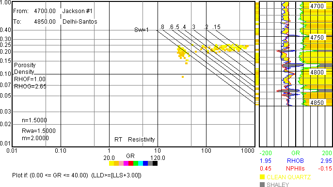
The water zone is now separated from the oil-bearing zone due to the filters. Note how the Sw lines are closer together with n=1.50 due to a lower Sw for a given resistivity. Reducing Rw, m or n reduces calculated Sw.
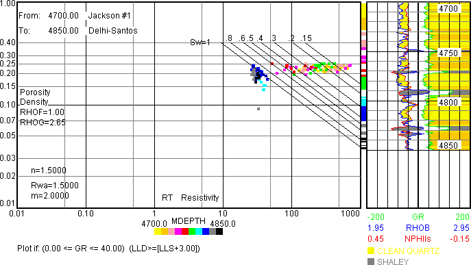
Note how it is possible to identify the top of the water zone at 4790 feet below the hydrocarbon bearing zone with measured depth (MDEPTH) in the Z-azis.
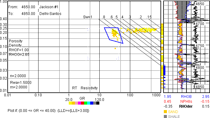
Use of the Trk 1 Logs (2 inch/100 ft) with Plots and Highlight Data in Plots features allow one to place the 4-sided polygon around the water-wet data cloud - water zone is flagged in blue at left edge of the Trk 1 Logs. Be sure to click the OK bar after dragging the Sw=1 line and the Done bar after making the polygon.
View Highlight Data menu item shows the results and that plot can then be saved as GIF file for further use with File/Save As.../GIF.
Note how Calculated Curve RHOmaa (RHOder) DIFF Differential based on depth increment, identifies sand-shale interfaces.
RHOG=2.65 and RHOF=1.00 can be set to compute Density Porosity for the Pickett Plot with the Models/Variables/Density Porosity... menu item.
Rmfa can be estimated with the Pickett Plot by selecting Pickett /Rxo instead of Pickett /RT and making the plot over the 4800-4850 foot interval. Rmfa=0.45 for and m=2.0 are reasonable. Click on the OK bar at the very bottom when finished.
Four filters in total are available. The Delta filter is very useful in some cases as seen above.
Use this characteristic to select only the permeable rock in various plots. Try some Litho plots with the Delta Filter.
Rxo-RT Plot... is a way to estimate Rw and Sw without a porosity log. It works well in carbonates.
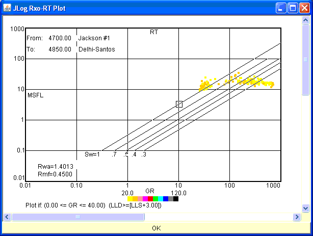
Rwa=1.4 when Rmf=0.45 above. Note the use of the GR and Delta filters. Be sure to click the OK bar after dragging the small target so the Sw=1 (Sw=100%) line passes through the water data. After the user clicks on the OK bar at the bottom of the plot the resulting Rwa is recorded. See the a, m, n, Rw and Rmf... menu item of the Models/Variables submenu to check for yourself.
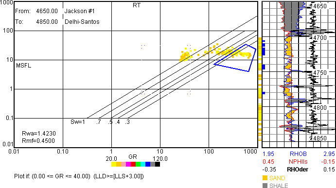
Use of the Trk 1 Logs with Plots and Highlight Data in Plots features allow one to place the 4-sided polygon around the best pay (lowest Sw) data cloud. Be sure to click the OK bar and Done bars as they appear.
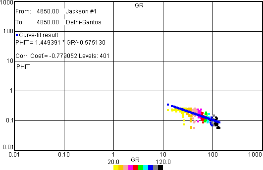
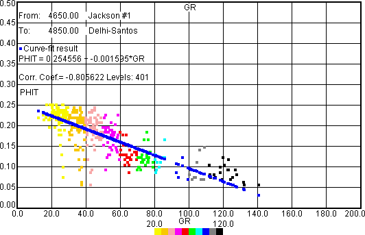
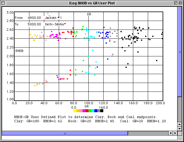
Six plots are available under the User submenu. User Defined Plot... plots one log or Calculated Curve vs. another in either linear or logarithmic scale. Linear and power curve fits are available.
In this User Defined Plot... RHOB and GR values are plotted below to select Clay, Rock and Coal endpoints used to determine Eval lithology track
mineral volumes in the Clay Rock Coal Eval Mineral Model. All filters are off.
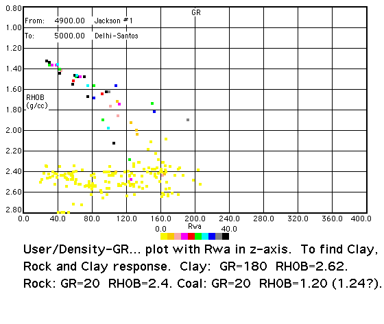
Above, with Density-GR... of User submenu one plots Density vs. GR in linear scale. RHOB and GR values are plotted here to select Clay, Rock and Coal endpoints used to determine Eval lithology track
mineral volumes in the Clay Rock Coal Eval Mineral Model. This is faster and easier than setting up the User Defined Plot... shown just above.
The following PHID-GR... plot aids in identifying laminated sand-shale layers for the Thomas-Stieber model.
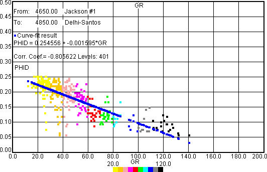
PHID (density porosity) above is computed with RHOG=2.65 and RHOF=1.00.
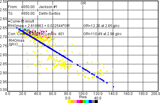
RHOmaa-GR... of User submenu plots RHOmaa vs. GR in linear scale. Both RHOmaa and GR values are plotted here to select clean and clay or shale endpoints as explained by Robert Elphick years ago.
This is faster than setting up the User Defined Plot... above. The clean and clay GR and RHOmaa values can be used in VclayGR and VclayRHOB-NPHIls of Models/Which Vclay?... later. This plot is also used to check for hydrocarbon effects in shaly sands - gas in particular will fall above the trend with possible, increasing Rwa.
Here GR endpoints for Vclay or Vshale are estimated for 2.65 (sand) and 2.90 (clay or shale) endpoints.
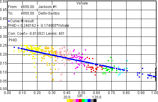
Above, with PHID-Vshale... of User submenu one plots PHID vs. Vshale from VshaleGR (GR clean=8 GR shale=105) in linear scale. This aids in PHIsand and PHIshale estimates for Thomas-Stieber model worked later.
Vshale-Rt... of User submenu is based on a concept from Dick Merkel that aids in Rshale selection and Vshale indicator quality for the Indonesian Sw model. Dick has found that a plot of Vshale (y-axis) against RT (x-axis) should yield a slope of -1 when the Vshale indicator is valid. This feature is intended for the Eval 1-Mineral (clean or clayey) model that needs a shaly sand indicator. It is also useful in estimating Rshale for the T-S (Thomas-Stieber) laminated sand-shale model.
If Indonesian Sw model Rshale is needed later from mineral 3 volume for Vclay of Eval 3-Mineral PEF or 3-Mineral Sonic select VclayRHOmaa-Umma or VclayRHOmaa-Tmaa.
Rshale can be estimated at Vshale=1. I am still experimenting with this concept and so far it is clear that some Vshale indicators need improvement. This method is better than "eye-balling" Rshale from the logs which seems to over-estimate Rshale values. Instead of an eye-balled Rshale of 10 it appears that Rshale at 3 is more appropiate for the Niobrara example below. Lower Rshale leads to lower Indonesian Sw values.
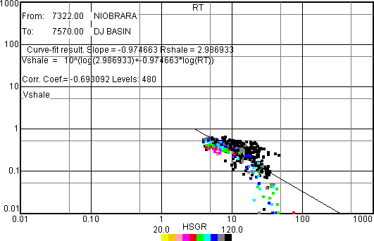
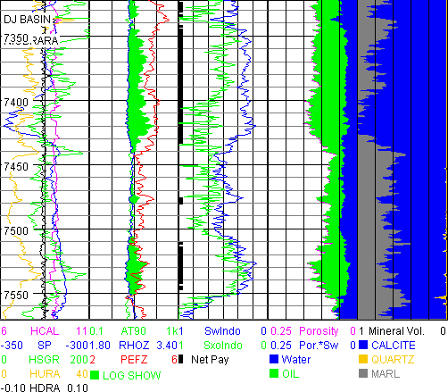
Below is the Indonesian Sw model with Rshale=3 applied to the Niobrara example. Note PEFZ increase at the top (pyrite?).
The Trk 1 Logs with Plots menu item allows one to plot Track 1 logs to right of the crossplot. Z-axis data color will be plotted just to the right of the crossplot to help correlate crossplot data with depth and Track 1 logs. Track 1 Logs depth scale is set when plotting logs.
For Litho and Source Rock crossplots it is possible to Highlight a data group or cloud within a user-selected four-sided polygon by selecting Highlight Data in Plots, making the crossplot, dragging the four little corner targets and clicking on the Done bar when finished. Selecting View Highlight Data will show the blue thick line polygon and the blue ticks at the left edge of the log plot that marks data within the four-sided blue polygon. This plot can be saved as a GIF or other graphic file type with File/Save As... in the normal manner. Eval/Sw-PHI... and Sw-PHI with Perm... can be highlighted in the same way.
Pickett and Rxo-RT plots can also be highlighted as demonstrated earlier.
The Histogram... menu item allows one to make a histogram of a log or Calculated Curve in a user defined color and in a user defined number of bins. This can be useful when scaling log curves for the User Defined Plot... .
Section V: Models Menu
Mineral Models, Vclay, Vshale, Porosity, Sw and Variables that affect those models are selected. Overrides allow the user to squeeze more out of a limited data set. Logic is available to identify coal and to utilize sonic porosity in bad hole.
Twelve Eval Mineral Models are available in addition to coal detection and 6 overrides.
Lithology, Source, Pickett, Rxo-RT and other plots aid in lithology and fluid identification and should be made to aid in model selection.
Local knowledge, mud log, cuttings, core description, XRD and Rock-Eval should also be used to aid in model selection.
It is critical that the selected model matches the rocks and fluids within.
JLog menu progession from left to right and top to bottom is such that once a model has been selected, unneeded menu items will be blanked off. If 2-Mineral (clean carbonates)... is selected there is no need for Vclay so Which Vclay?... is blanked out.
Minerals can be named within the models and with Eval/Paint Minerals & Fluids... This is where one can change mineral names such as CLAY to SHALE or MARL and so on. Mineral colors are changed here also if one does not like the model assigned color.
1-Mineral (clean or clayey)... is a shaly sand model appropriate for SAND.TXT. The Indonesian and Dual Water Total and Effective Sw equations, among others, could be used here in addition to Archie.
Thomas-Stieber (laminated sand)... is a shaly sand model appropriate for laminated (the dispersed shale model is not implemented here) sand-shale reservoirs where the sand and shale laminations are thinner than the log resolution and where the lower shale resistivity is masking the higher hydrocarbon-bearing sand resistivity. This T-S model adaptation is based on: Thomas, E. C. and Stieber, S. J., 1975, The Distribution of Shale in Sandstones and its Effect upon Porosity: SPWLA 16th Annual Logging Symposium, June 4-7, 1975. It is very important that this paper be read before using the T-S model. Parallel or Series model resistivity can be selected along with a Calculated or Constant clean-sand porosity.
This model applies Archie Sw to the clean sand lamination porosity using Rsand and PHIsand to obtain SwTSlam of the clean sand lamination. Rsand is estimated from RT resistivity corrected for Rshale and Vshale while PHIsand is either an input Constant (constant porosity for each lamination) or Calculated from Density porosity (PHID) corrected for PHIshale and Vshale.
PHID=(RHOG-Density)/(RHOG-RHOF) is not corrected for Kerogen or pyrite.
PHIsand hydrocarbon volume is multiplied by (1-Vshale) to estimate in place hydrocarbons. It is very important to have geologic input to be sure this model, and all models, apply to the actual rocks. The model was designed for a GR based Vshale estimate.
2-Mineral (clean carbonates)... is appropriate for carbonates. The user supplies the grain density (RHOG) of each carbonate. Typically this would be 2.71 for limestone and 2.85-2.87 for dolomite. Both density and modern neutron logs such as NPHI, CNC and TNPH are required for this model. An old NEUT in counts/sec would not be suitable unless it had been recalibrated to limestone porosity units. The Constant, Ratio and Archie Sw equations could be used here. This model is appropriate for CARB.LAS. If a compressional sonic is available Khoyle (carbonate permeability indicator) may be plotted to assist in the identification of permeable carbonates. Khoyle makes use of the fact that compressional velocity often increases with increasing carbonate permeability. Reference: Hoyle, W. R. and Bowler, J., 1998, Wyllie Revisited with Respect to Carbonate Permeability: The Log Analyst, Jan-Feb 1998. Khoyle may read too high in oolitic and oomoldic carbonates.
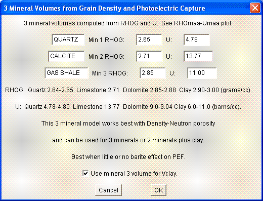
3-Mineral PEF... is appropriate for carbonates, mixtures of 3 clean minerals or a mixture of 2 minerals plus clay or shale. The user supplies the grain density (RHOG) and U of each mineral. Density and modern neutron logs such as NPHI, CNC and TNPH along with photoelectric capture cross section (PEF, PE) are required for this model. An old NEUT in counts/sec would not be suitable unless it had been recalibrated to limestone porosity units. Mineral 3 can be Clay or Shale and a shaly sand Sw equation could be used with Vclay or Vshale from mineral 3. This model is appropriate for SAND.TXT and CARB.LAS. Barite in the mud may create problems with this model due to an increased PEF and U.
3-Mineral Sonic... is appropriate for the same mineral mixes as 3-Mineral PEF... but uses sonic instead of PEF. The user supplies the grain density (RHOG) and Tmaa of each mineral based on the MID plot. This model can be used when barite affects the PEF but is not always as good a lithology indicator as the 3-Mineral PEF. Mineral 3 can also be used for Vclay or Vshale.
4-Mineral (clean carbonates)... is appropriate for quartz, calcite, dolomite and anhydrite or pyrite lithology and clay-free rocks. Density-Neutron porosity is preferred but other porosity models can be used with care. Either Constant, Archie or Ratio Sw is available.
5-Mineral (carbonate + clay)... is appropriate for quartz, calcite, dolomite, clay and anhydrite or pyrite lithology. Density-Neutron porosity and all the JLog Sw models are available.
The Sand Silt Clay... model uses Density and Neutron values determined from the Density-Neutron crossplot along with Sand and Silt grain density values. Density Porosity is estimated from the log density value and user Sand and Silt grain density selection. Vclay is estimated from the 3 mineral volume solution based on each of the 3 mineral density-neutron pair values input by the user.
The Clay Rock Coal... model uses the density log and GR to estimate gas in place from a scf/ton Desorption=a+b*Curve^c relationship. a, b and c are estimated from coal core desorption data related to a log curve which is usually the density. The relationship is determined by JLog or spreadsheet curve fitting of lab desorption data to the log Curve (usually density). A density vs. GR User Plot determines the 3 Clay, Rock and Coal endpoints. scf/ton means standard cubic feet of gas/ton of coal - scf gas volume is at 14.7 psi and 60 F (15.6 C). One ton is 2,000 pounds.
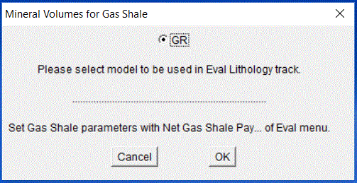
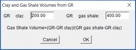
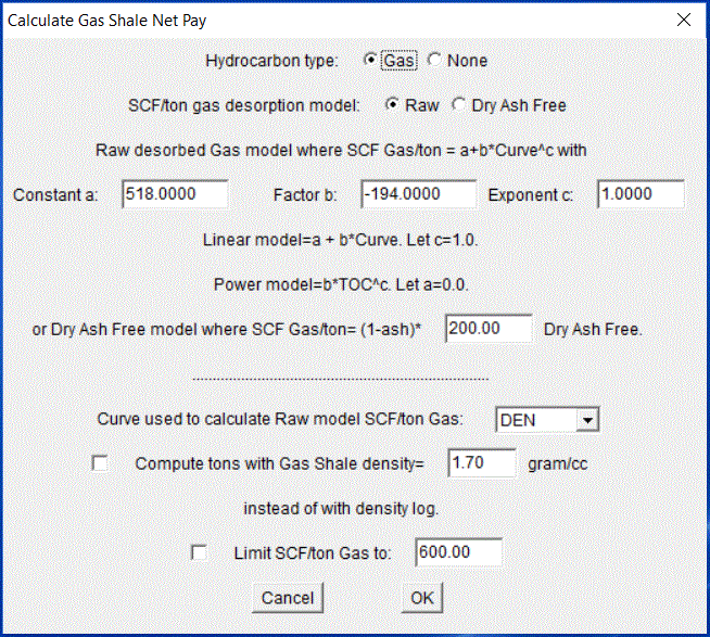
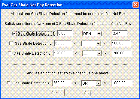
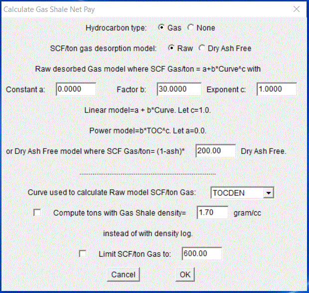
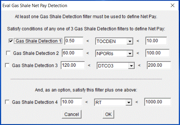
Gas Shale... uses 5-mineral and two 3-mineral models to estimate quartz, calcite and Gas Shale content or just GR to estimate Clay and Gas Shale volumes. If the relationship between scf/ton and TOC is known then gas in place can be computed or a desorption relationship similar to that in the Clay Rock Coal model can estimate gas in place.
Source Rock... uses the same Gas Shale lithology models plus a 2-Mineral model. Passey delta log R Total Organic Carbon (TOCDLR), Haecker density (TOCDEN) or curve for TOC. S1 and S2 (mg hc/g rock) may also be estimated from this TOC if lab data is available for calibration.
Pulsed Neutron... uses Sigma and a porosity log or curve to estimate hydrocarbons in place for Clean or Clayey (Shaly) reservoir rocks.
Coal Detection... is available for some models and may be triggered by any one of 3 user selected logs. A Coal count can be presented in the Eval Net Pay summary.
Porosity/Mineral Override... Six overrides are available and are designed to squeeze more from the logs by substituting another porosity and lithology model when appropriate. Vclay (Vshale) is set to zero and Porosity is selected when an override is called. This feature is useful when evaluating carbonates with a minimal set of logs by setting Override 1 as 50 less than GR less than 1000 gray SHALE. Override 2 as 2.88 less than RHOB less than 1000 cyan ANHYDRITE for anhydrite. The Constant override porosity model with porosity=0.0 is appropriate for both.
Care must be taken not to override permeable radioactive carbonates. Everything that is radioactive is not shale or clay.
Override Porosity will apply to Pickett Plot Porosity when making a Pickett Plot so be careful.
Experiment with this feature to find out what it can do.
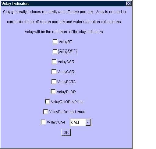
Which Vclay?... allows a selection of Vclay indicators, as above, needed to calculate Indonesian, Dual Water Total and Effective Sw for 1-Mineral (clean or shaly) and Sigma Clay Sw in the Pulsed Neutron model. Vclay will be the minimum of the clay indicators which are computed at each depth. Nothing has yet been selected here. If a Vclay curve such as VclayRHOmaa-Tmaa is unavailable due to an absent curve (sonic in this case) it will not appear as a possible clay indicator. Any curve may be selected for VclayCurve. Here the caliper is shown for VclayCurve because in some cases the hole is at bit size in clean sands and badly washed out as clay content increases. The checkbox is yet to be checked to take effect as a Vclay indicator. Clean and clay values are set under the appropriate Variables of the Models menu.
Which Vclay?... will be "grayed out" except for 1-Mineral (clean or clayey)... and Pulsed Neutron... of Eval Mineral Models that use a Vclay from Which Vclay?...
JLog 10 and above attempt to use a more appropriate terminology for Indonesian and T-S water saturation models. Vclay and clay terms are changed to Vshale and shale.
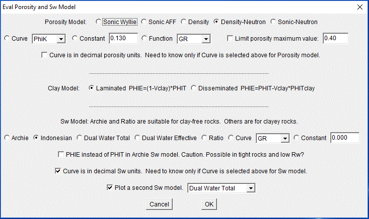
Porosity & Sw Models... :
Porosity can be selected from models such as Sonic Wyllie, Density-Neutron, Microlog and so on. Available choices depend on logs present. If a porosity log such as Density is absent, then Density and Density-Neutron options will be absent. One can also select a Curve to be the porosity log (JLog needs to know if the Curve is in decimal porosity units or not). The Curve porosity can be from another log or it may be PhiK % when dealing with oil-prone Type II marine kerogen - be sure to leave "Curve is in decimal porosity units" unchecked for PhiK as it is in % - % units will be converted to decimal for use in JLog. If no porosity logs are present it is possible to set porosity to a constant value. Porosity may be limited to a maximum value which is useful in bad hole where porosity may read too high and result in false shows.
Here Density-Neutron porosity is selected.
Two clay models relating Vclay and total porosity (PHIT) to effective porosity (PHIE) are available. The Laminated model is selected.
Seven Sw models are available. The Indonesian Sw model is selected. The Dual Water Total model has also been selected for comparison which can be very useful for final Sw model determination as both will be plotted. Curve is an imported Sw from an outside source. Sw Constant of 0.000 is meant to be used with source rock kerogen PhiK porosity that is expected to be 100% oil saturated.

The Ratio model is normally used for clean carbonates with an exponent of 0.625 that can be modified with caution. The model does not need a knowledge of m and n. Although it is designed for use with PHIT it can be used with a Vclay indicator and PHIE for reserve calculations.
Bad Hole Sonic Porosity... is available if there is a sonic log. Since the sonic is often the most robust of the porosity tools it can be called for use in bad hole situations. For example in an 8.5 inch hole you might want to use the Sonic Porosity AFF Model whenever the hole was greater than 12 inch. To do this just check "Bad Hole Trigger 1" checkbox and set 12 < CALI < 100. Whenever the caliper (CALI) is greater than 12 inches the sonic will be used for porosity. The CALI is not likely to read greater than 100. You can show where the sonic has been used on the Eval graphic plot by checking Show Eval Sonic Porosity Flag which will appear as a green mark at the right edge the Eval/Plot Eval Sw track.
The Variables submenu is used for setting variables such as a, m, n, Rw Rmf, Density and Sonic porosity paramaters, PHIT and RT clay, GR clean and GR clay for Vclay from GR and so on for other clay or shale indicators. Which RT?..., Which Rxo?... and Which Sigma... allow selection of any curve for RT, Rxo and Sigma. This can be useful if there is more than one curve in the incoming LAS or TXT file that can be used for RT or Rxo.
Section VI: Eval Menu
The evaluation hydrocarbon reserves are estimated here after the appropriate model and variables are set earlier. Results are displayed graphically and in text on the screen with a reservoir summary.
Calculated Curves such as Rwa, TOCDLR and S1 may be plotted along with logs. Eval answers including Vclay, Porosity and Sw are computed at each depth level and may be saved in LAS and TEXT files along with the reservoir summary in TEXT for report writing. The LAS file can be imported by other applications for further use.
Working from top to bottom in the normal JLog manner the Net Pay... menu item allows one to estimate predominately Oil or Gas reserves or None. Vclay, PHIE (effective porosity) and Sw (water saturation) cutoffs are set when appropriate. If the Archie Sw model is used the Vclay cutoff has no effect unless a Vclay indicator has been selected. Vshale cutoff can be set just above 1.0 and below 1.10 to count all shale in Net Pay if need be when working with unconventional reservoirs. When Eval calculations meet the cutoff conditions Net Pay and Net Reservoir will be counted. The Net Pay flag appears in the Sw track of the Eval plot. These Net Pay intervals might be perforated if not too close to water.
The Vclay term becomes Vshale in JLog version 10 for Indonesian and T-S Sw models.
It is possible to filter Net Pay on a log or Calculated Curve with up to 4 filters plus a Delta Filter. Perhaps Net Pay should only be counted if the GR is less than or equal to (<=) 25. In this case the "Net Pay if" checkbox is checked and 0.0000 <= GR <= 25.0000 would be input. From: and To: depths would be input over the interval where this filter would apply (not done here).
In the next dialog are 3 more filters plus a Delta Filter that may be applied (not done in example below). This gives plenty of filter capability.
In the next dialog are a number of factors needed to compute reserves such as drainage area acres, formation volume factor and recovery factor as appropriate.
Calculate Quick Net Pay... does exactly that. Input the From: and To: interval and you will rapidly obtain a Net Pay and Net Reservoir summary based on the models and variables you have selected.

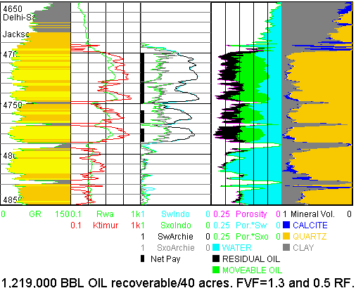
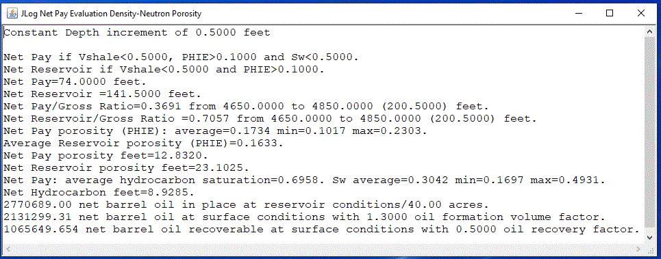
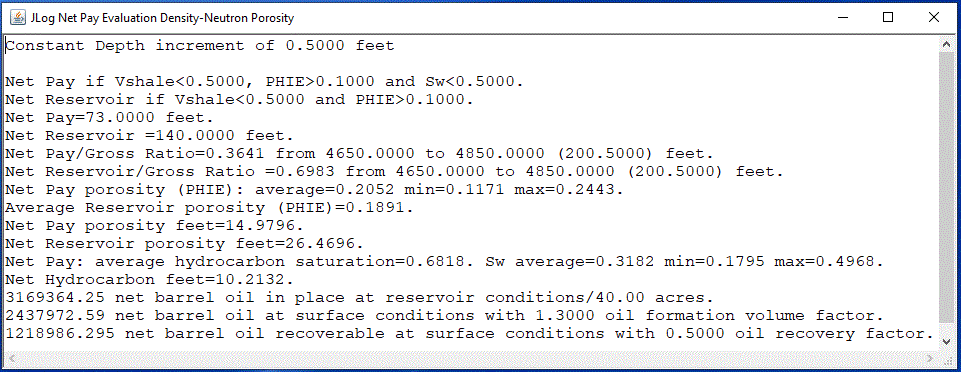
Here is a typical Quick Net Pay summary from Jackson#1.JLG with Eval Mineral Models/1-Mineral (clean or shaly...). Notice the estimate of barrels of oil recoverable at surface based on the user input of drainage area, formation volume factor and recovery factor.
The Net Pay summary can be copied and pasted into a document or other application for presentation.
The Evaluation included the following models and variables using shale terminology introduced in JLog 10 for Indonesian Sw. VshaleGR with clean=8 and shale=105. Density-Neutron Porosity, Laminated shale, Indonesian Sw, RTshale=26, Rw=1.4, Rmf=0.45, m=n=2 and a=1.0.
View Eval Answers... lists all the variables and equations used in the evaluation in the upper split window (always check the models and variables here before finalizing the evaluation) along with a Net Pay and Net Reservoir summary with up to 1000 level by level answers. This model, variables information and as many as needed, level by level answers can be saved with Save As... of the File menu. Choose and push "Eval in TEXT" button to do so. Answers can also be saved as LAS for export to other software with Logs and Eval in LAS. Calculated Curves may also be saved.
Eval colors and names for minerals and fluids are set with Paint Minerals & Fluids... of the Eval menu. Gas-Oil contact depth and gas colors and names can be set here to color gas above oil.
Eval presentation is set with Setup Eval Tracks... of the Eval menu.
Plot Which Calculated Curves... of the Eval menu sets up the plotting of various Calculated Curves such as phiS, phiND, RHMA, Rwa, Rmfa, PHIT, PHIE, Vclay, Sw, Sxo, BVW, BVH, Ktimur, Ro (100% water-wet resistivity), TOCDLR, DlogR, TOCDEN, FOIL and SwFoil if the appropriate logs are available. phiS is sonic Wyllie porosity computed from the matrix travel time estimated from the matrix density (RHMA) determined from the density-neutron crossplot. phiND is density-neutron crossplot porosity. PHIT is total porosity determined from the porosity models selected from Porosity & Sw Models... of the Models menu while PHIE is the resulting effective porosity after Vclay correction. Vclay will be the minimum of the clay estimators from Which Vclay?... of the Models menu. Rwa=Rt*PHIT^m. Rwa a is a good quick look hydrocarbon indicator. Rmfa=Rxo*PHIT^m. Rmfa can identify hydrocarbons in clean formations with changing and fresh Rw values. Often Rmfa in the hydrocarbon zone will be about twice that in the water zone. Remember that Vclay will become Vshale for Indonesian Sw and the T-S model.
See JLog Calculated Curves.pdf for a description and an explanation for the growing number of Calculated Curves.
The Eval graphics plot is made with Plot Eval of the Eval menu with standard and user defined depth scales.

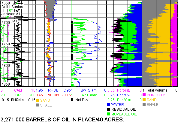
Note the black bar at the left edge of Track 3 which flags Net Pay in the Eval plot above. Note also the shading between the RHOB and NPHIls curves which show the quartz and shale effects on these 2 logs.
Sw-PHI... and Sw-PHI with Perm... identifies the best reservoir and perhaps estimates permeability. Permeability here should be thought of as qualitative not quantitative. PHI denotes porosity.
And here is the Sw-PHI with Perm... plot for the Eval plot above.
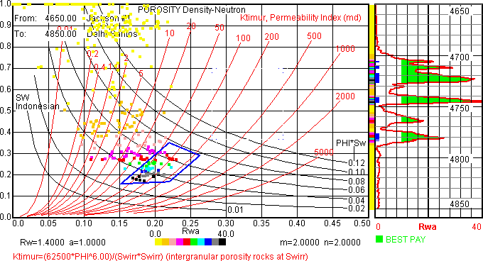
Note the data cluster bounded by the blue polygon and 50 to 200 Ktimur permeability lines. They identify the better reservoir which generally has higher Rwa values seen opposite the blue flags of Trk 1 Logs. This plot is very useful for selecting Porosity and Sw Net Pay cutoffs and for comparing evaluations well-to-well.
Next will be Thomas-Stieber model evaluation based on the following two User plots that suggest the Jackson #1 sands are laminar.


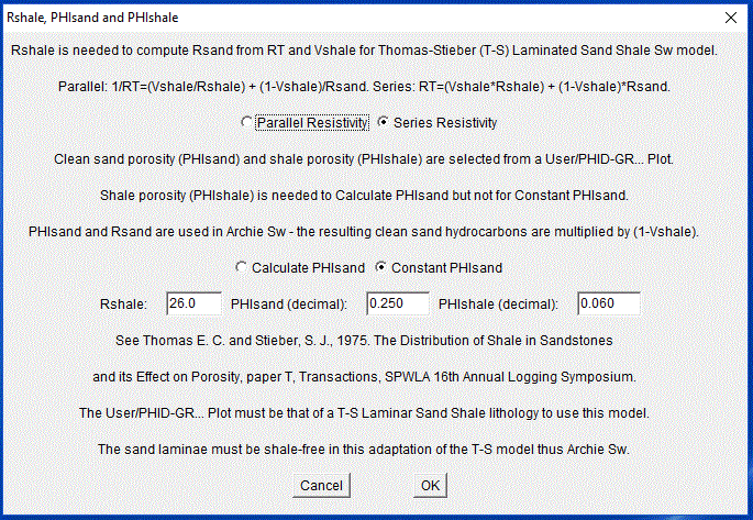
The two plots suggest a clean sand porosity (PHIsand) of 0.25 (25%) to be used for the Thomas-Stieber (T-S) model - Constant PHIsand adaptation that assumes that each clean sand lamination has a constant 25% porosity.
This is where geological knowledge of the rocks is required. That is the case for all models - lithology and source rock plots can help.
With Models/Eval Mineral Models/Thomas-Stieber (laminated sand-shale)... check the VshaleGR box as that is the normal Vshale indicator for T-S. Another shale indicator may be appropriate if radioactivity is due to non-clay minerals such as mica.
Models/Variables/GR clean & shale... are used to set GR clean and GR shale in the normal way.
The Constant Porosity PHIsand (0.25) model and Series Resistivity for laterolog are selected below. The Parallel Resistivity model would be appropriate for an induction resistivity.
The T-S Eval plot (0.25 PHIsand Constant Porosity - Series Resistivity) that follows has the same evaluation variables as in the previous 1-Mineral model that used Density-Neutron porosity and Indonesian Sw.

The T-S Calculate PHIsand model with Shale porosity (PHIshale) of 0.06 (6%) yields 3,818,000 BBL OIL/40 acres. PHIshale is always greater than 0.0. Reverting to the previous Constant Porosity (0.25) model, now with GRclean=12.20 and GRshale=110.49 (see earlier RHOmaa-GR plot) yields 3,486,000 instead of 3,271,000 BBL OIL/40 acres.
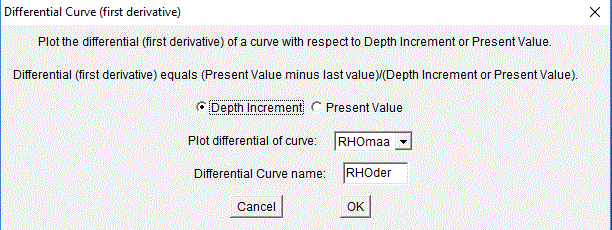
The (DIFF) differential of RHOmaa (aka first derivative) Calculated Curve is named RHOder and is plotted above in Track 1. Note the denominator may be the Depth Increment as selected below or the Present Value.
Next comes a 3-Mineral PEF Eval plot similar to the Jackson #1 Eval plot above that is derived from SAND.TXT. Here Vclay comes only from mineral 3 volume (RHOG=2.90 and U=6.5) from RHOmaa-Umaa plotted earlier. Be sure to check "Use mineral 3 volume for Vclay". Quartz and Calcite RHOG and U defaults are used. Rw=1.50.

Note Calculated Curves Rwa and Ktimur permeability in Track 2. Ktimur is computed with E=6.0 and C=62500.
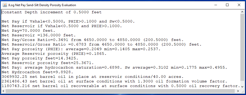
Here is the Quick Net Pay... summary for the Eval plot above.

Next comes a 2-Mineral Eval plot below generated from the CARB.LAS file with NPHI as the neutron log. CARB.LAS is a set of Schlumberger Platform Express (PEX) logs so NPOR, TNPH and NPHI neutrons are available in decimal limestone units (V/V). The CARB.LAS file was imported using import curve names for PEX. This LAS file contains many of the necessary variables such as Rm, Rmf etc. Rw=0.022 and Rmf=0.109 at reservoir temperature are used for this evaluation. The first two overrides are used starting with default values to depict SHALE and ANHYDRITE. The shale value was changed to 100 because porous zones with mudcake have high GR just below 100. Care should be taken when setting GR overrides so one does not eliminate radioactive, porous, permeable carbonates - the Khoyle carbonate permeability indicator (Calculated Curve) can help. Both override porosity models are Constant=0.0.
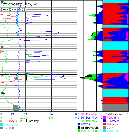
Note how CLAY and ANHYDRITE overrides above extend the 2-Mineral lithology model in the lithology track at the far right.

The 3-Mineral PEF model above comes next. The Eval plot now computes Anhydrite volumes. RHOG=2.90 and U=15.0 are used in place of Quartz for ANHYDRITE. Defaults are used for LIMESTONE and DOLOMITE. The ANHYDRITE override is not needed now while the CLAY override remains.
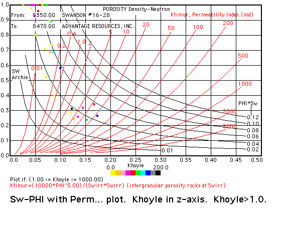
Sw-PHI... and Sw-PHI with Perm... identifies the best reservoir and perhaps estimates permeability. Ktimur and Khoyle in the Z-axis suggest some permeability is present.
The 3-Mineral Sonic model is next and is similar to the 3-Mineral PEF model except the MID plot is used to select the three lithology endpoints from RHOG and Tmaa.
The 4-Mineral (clean carbonates) model comes next and is an extension of the 3-Mineral PEF model for clean rocks so only Constant, Archie or Ratio Sw. Data outside the Quartz-Calcite-Dolomite RHOmaa-Umaa triangle that falls to the right of Calcite-Dolomite line and inside the Calcite-Dolomite-Anhydrite triangle can be quantified as a fourth mineral lithology - Anhydrite, Pyrite or something else based on user RHOG and U input. This 2 triangle lithology model is based on an AAPG Geobyte article by Robert Elphick. It is designed for Density-Neutron porosity but another porosity may be used if there is good reason to do so. Experiment to see how this works.

The 4-Mineral (clean carbonates) example above is set up with the default RHOG and U values for 4 mineral volumes with Anhydrite as mineral 4. Variables are set as in JLog Workflow Example for 5 Minerals that is found at the end of these instructions. There are two issues with the model selection that are improved in the 5 Mineral Workflow. Firstly: the caliper (HCAL) shows washed out borehole just above 8200 that causes a false porosity answer that results in a false log show over the enlarged borehole interval. Secondly: the SP and the GR suggest the intervals with increased GR and positive SP are likely to be shale and clay-rich. An improved evaluation that more accurately expresses lithology and pay is made with the 5-Mineral (carbonate + clay) model and an override - see JLog Workflow Example for 5 Minerals that follows later.
The 5-Mineral (carbonate + clay) model comes next. This lithology model is based on the Elphick 2 triangle solution applied to the McGinley and McKnight "Log-Derived Stratigraphic Reservoir Description" (1984 SPE 12597) model for quartz, limestone, dolomite and clay where dolomite and clay volumes depend on the sonic. Designed for Density-Neutron porosity and all Sw models. See the JLog Workflow Example for 5 Minerals at the end for more on this model.
Next comes a Sand, Silt, Clay model with 3 mineral volumes calculated from RHOB and NPHI endpoints selected in the Density-Neutron Plot shown above in Section IV: Plots Menu. This is not a good example but we will use it. The Sand Silt Clay lithology mix exhibits a boomerang or banana pattern based on the 3 minerals. This model is designed to allow silt to be included as a reservoir which may result in more Net Pay. The model seems to move in the right direction with an additional 300,000 barrels of oil in place over the 1-Mineral (clean or shaly) shaly sand model evaluation made earlier.
After selecting Sand Silt Clay... Model the following endpoints are used: Clay: NPHI=0.30 RHOB=2.50. Sand: NPHI=0.22 RHOB=2.20. Silt: NPHI=0.15 RHOB=2.45. Sand Grain Density=2.65. Silt Grain Density=2.71. Indonesian Sw, Laminated Clay with Rtclay=26, Rw=1.4, Rmf=0.45 and m=n=2.0 and a=1.0.
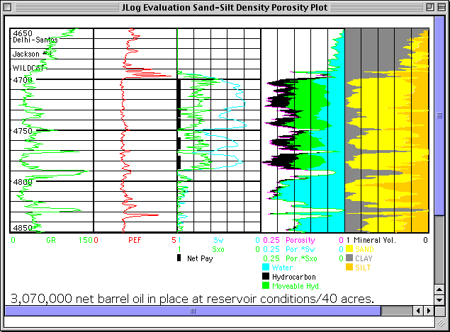
The Quick Net Pay Summary looks like this:

Next comes a Clay Rock Coal... model with 3 mineral volumes calculated from RHOB and GR endpoints selected in the RHOB vs. GR User Defined Plot... or the Density-GR... plot shown above in Section IV: Plots Menu. SCF*10^3 is posted at the left edge of Track 4 and coal thickness (Thick) at the right edge for each coal.
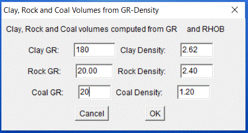
DESscf Eval/Calculated Curve is 20.0 + 200.0*RHOB^-4.2 and is placed in track 2. This relates total lab desorbed gas (DESscf) in scf/ton to the bulk density log. Make a table with lab total desorption (DESscf)in one column and log bulk density (RHOB) value in another and fit DESscf to RHOB. Depth matching coal sample depth to log depth is important. Generally DESscf increases as RHOB decreases in a coal.
Then with Eval/Net Coal Gas Pay... set up as follows for 40 acres drainage.

Use RHOB<2.20 to detect coal as follows. The RHOB-GR plot can be used to select the RHOB cutoff. In this case 2.20 can be seen to include adjacent shales or clays that also contribute gas.

The Eval/Quick Coal Gas Net Pay... summary looks like this with the hypothetical Scf/ton relationship to RHOB:
Depth increment = 0.5000 feet.
Net Pay = 20.5000 feet.
Net Pay/Gross Ratio = 0.2040 from 4900.0000 to 5000.0000 (100.5000) feet.
Coal detected when one of the following conditions is satisfied:
0.00 < RHOB < 2.20.
87.03*10^6 net cubic feet of gas in place at surface conditions/40.00 acres.
RHOB density curve in gram/cc used to compute tons in scf/ton Gas.
Scf/ton= 20.0000 + 200.0000 * RHOB ^ -4.2000.
DAF=(Scf/ton)/(Coal decimal volume) when more than 1% Coal.
With Eval/Setup Eval Tracks... set as follows.

With Eval/Plot Eval/5 inch/100 ft (1/240)... make the following. SCF*10^3 is posted at the left edge of Track 4 and coal thickness (Thick) at the right edge for each coal.

The Gas Shale model determines gas reserves from a relationship between desorption or total gas in scf/ton and a log or a Calculated Curve. This relationship needs to be determined from lab and log data. If an average scf/ton is known that can be used. Gas Shales generally have high GR, lower bulk density and higher resistivity than other shales. This results in a higher Rwa (Rt*porosity^m). At the minimum, a GR log is needed to estimate Gas Shale volume in the lithology track.
Step by step Eval/Gas Shale... model instructions follow for two wells - the first with an older log set over the New Albany Shale where GR is used to try to identify Gas Shale in the Eval Lithology track.
Neither well is shipped with JLog.
1. Import data in the normal way with File/Import.
2. After checking data import with Logs/View Log Values.... and Plot Logs select Models/Eval Mineral Models/Gas Shale... . GR, 3-Mineral PEF, 3-Mineral Sonic and 5-Mineral lithology models may be used if the appropriate logs are available.
First the GR, the only lithology model available before JLog version 6 will be described using a relationship between SCF/ton and the bulk density (DEN) log.

Enter the GR clay and GR gas shale values. The equation used to compute Gas Shale volume is displayed in Eval Lithology track is displayed in the dialog below. Any GR above 200 is to be due to Gas Shale.

3. With Eval/Net Gas Shale Pay... enter the SCF Gas/ton relationship, drainage area and select a filter to define Net Pay.


4. The rest of the evaluation is carried on in the normal way. Use Eval/View Gas Shale Answers... over 10 feet to check models in the upper split window.
5. The Eval/Calculate Quick Gas Shale Net Pay summary looks like this:

6. Eval/Plot Eval at 5 inch/100 feet (1/240)... gives the following plot.
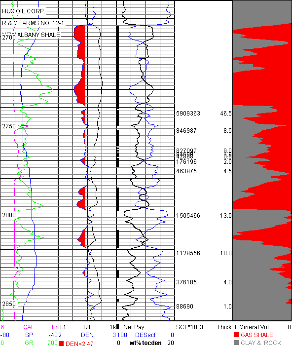
11.5 BCF GAS Net Pay in place at surface conditions/section.
IPF: 100 MCF @ 1,050 PSI through 3/4" choke (2,698-2,738 feet).
Haecker TOCDEN for New Albany Shale presented in track 3 as wt%tocden with a=158.01 and b=58.44.
7. Here is a Niobrara, 3-Mineral PEF, example with a hypothetical relationship between SCF/TON gas and TOC calculated with Haecker TOCDEN Niobrara parameters. First plot TOCDEN (without Filter TOC) Calculated Curve as explained in part C: Density Correlation method of the Source & Tight Oil Manual 11 with Niobrara parameters of a=144.18 and b=54.54 - these values are not far from those of the All North America Formation. Then select Models/Eval Mineral Models/Gas Shale... .
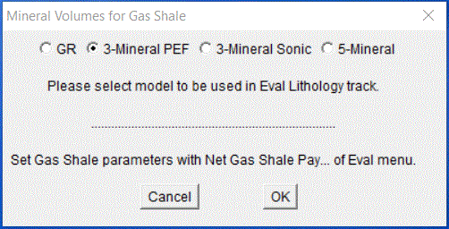
8. For the Gas Shale... 3-Mineral PEF example QUARTZ and CALCITE names and default values are used. GAS SHALE RHOG=2.85 and U=11.0 are estimated from the RHOmaa-Umaa plot.

9. At this point the lithology model for the Eval Lithology track is set up just like it would be in a 3-Mineral PEF Eval model.
TOCDEN is calculated using the Haecker TOCDEN method explained in the Source & Tight Oil Manual. A simple hypothetical relationship between scf/ton gas and TOC is to be used with Haecker TOCDEN Niobrara parameters of a=144.18 and b=54.54.
10. With Eval/Net Gas Shale Pay... enter the SCF Gas/ton to TOC relationship in the dialog below (don't forget c: 1.00), 640 acres drainage area and select a Gas Shale Net Pay filter so only TOCDEN>0.5 is used to compute gas in place.

The relationship between scf/ton and TOC is scf/ton=30*TOC. TOC is from TOCDEN Calculated Curve. The TOCDEN Gas Shale Net Pay filter below is applied so gas in place will only be calculated when TOCDEN>0.5.

11. The Eval/Calculate Quick Gas Shale Net Pay... summary follows below.

12. Eval/Plot Eval at 5 inch/100 feet (1/240)... gives the following plot over a short section of the pay.

118 perf holes 7290-8482 feet. 24 hour test flowing. CALC 1050 MCF GAS CALC 17 BBL WATER. 1500 tubing pressure 1750 casing pressure.
The Source Rock model includes calculations of S1 (free thermally extractable hydrocarbons) and S2 (present day source potential) converted to BBL Oil knowing API oil gravity. The separate Source & Tight Oil Manual is available for this model. Just open SourceRock.html in Source & Tight Oil Manual with a web browser where you will find step-by-step workflows for up to 6 Source Rock techniques plus tight oil identification methods and the infamous BRIT indicator.
Before working with the JLog Source Rock model and associated Calculated Curves it is recommended that one read Passey, Q. R., Creany, S., Kulla, J. B., Moretti, F. J. and Stroud, J. D., 1990, A Practical Model for Organic Richness from Porosity and Resistivity Logs: American Association of Petroleum Geologists Bulletin, v. 74/12, p. 1777-1794 and Haecker, Carvajal & White, 2016, Comparison of Organic Matter Correlations in North American Shale Plays: SPWLA 57th Annual Logging Symposium, paper Q.
The Pulsed Neutron model determines Sw from Sigma and works best in high formation water salinities. It is necessary to have both sigma from the pulsed neutron and a porosity log to solve for Sw in the Sigma Clean Sw model. A clay indicator such as GR is needed to find Sw in the Sigma Clay model. The clay indicator reduces total porosity to effective porosity in the usual way. Effective porosity (PHIE) is used in the Sigma Clay Sw model while total porosity (PHIT) is used in the Sigma Clean Sw model as in Archie Sw model because PHIE=PHIT.
If a clay indicator is selected with the Sigma Clay Sw model Clay, Mineral-1 and PHIE are displayed in the lithology track of the Evaluation plot. PHIE is in Track 4.
If a clay indicator is selected with the Sigma Clean Sw model then Clay, Mineral-1 and are PHIE in lithology track of the the Evaluation plot. PHIT is in Track 4.
If no clay indicator is selected with the Sigma Clean Sw only Mineral-1 and PHIT are displayed in Track 5 (lithology track) and PHIT in Track 4.
Step by step Pulsed Neutron model instructions follow.
1. Import data in the normal way with File/Import.
2. Sigma, Ratio, Near and Far counts and other Pulsed Neutron curves are placed in the 33 extra curves slots. When the "Add more curves?" dialog comes up push the "Add up to 33 more curves." button and add the necessary pulsed neutron curves including Sigma. Remember: the curve names are case sensitive and usually are upper case.
3. If Rw or formation water salinity is known Sigma Formation Water (Zw) can be found with Edit/Rw/Fluid Resistivity Calculator... .
4. After checking the data import values with Logs/View Log Values.... and Plot Logs you may wish to make Sigma-GR Plots/User plots to determine Sigma Matrix (Zma) and Sigma Clay (Zclay).
5. Models/Eval Mineral Models.../Pulsed Neutron.
6. Models/Which Vclay?... for a Vclay indicator in the normal way.
7. Models/Porosity & Sw Models... . Select porosity and Sw models here.
8. Variables/Zw, Zma, Zhyd and Zclay... . Plus appropriate Variables for Vclay and Porosity models are selected.
9. Models/Variables/Which Sigma?... to select the Sigma curve from which Sw is computed.
10. At this point a Sigma-Porosity User plot might be helpful to estimate Sigma Hydrocarbon (Zhyd).
11. The rest of the evaluation is carried on in the normal way. Use Eval/View Eval Answers... over 10 feet to check models and variables in the upper split window.
The FOIL (Cuddy et al., 1993, SPWLA Symposium, Paper H) Saturation-height Function shown below estimates BVW based on height (H) above Free Water Level (FWL). BVW(FOIL)=A*H^B where A and B are constants. Sw can be computed at any H: Sw=BVW(FOIL)/Porosity. JLog uses effective or total porosity.

FOIL constants A and B are suitable only for the petrofacies unit represented by the higher quality sands above. See Worthington 2002, Geological Application of Well Logs, AAPG Methods in Exploration Series No. 13, Chapter 7, for an excellent review on the use of Saturation-height Functions and the definition of a petrofacies unit. FOIL is for advanced users. A separate FOIL User Manual is available for the use of the FOIL model - just open satheight.html in FOIL User Manual with a web browser.
JLog Workflow Example for 5 Minerals
Here is an example of the workflow one might use to evaluate the dolomite pay in DOLO.LAS.
Import DOLO.LAS with File/Import in the normal way. This is a well written LAS file with NPHI, NPOR and TNPH in decimal limestone porosity units. With File/Reverse Depths... make a new JLG file since the LAS depths run from bottom to top and we want depths from top to bottom.
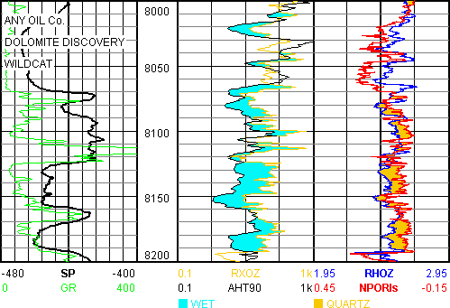
Plot the logs above with Logs/Plot Logs/2 inch/100 ft (1/600)... . Use Logs/Shade Between... as above. The increased negative SP suggests the formation water in the dolomite above 8070 is a bit more saline than that in the wet sands below 8070. It is clear from the lower, eyeball RXOZ/AHT90 ratio that there is pay above 8064.
Next identify lithology from a variety of cross plots.
Select NPORls with Plots/Which Neutron... since 3 neutrons are present in DOLO.LAS.
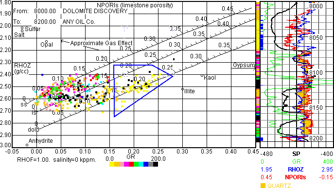
With Plots/Litho & Source Rock submenu make the Density-Neutron plot above after moving RHOZ and NPORls to Trk 1 with Logs/Plot Which Logs?... . Use Plots menu to place a blue polygon around a data cluster with Trk 1 Logs with Plots and Highlight Data in Plots. It appears that radioactive quartz sand with high GR (or chert) and good porosity clean dolomite (within blue polygon) are present after selecting Plots/View Highlight Data. This is an example where GR is not a good clay or shale indicator.
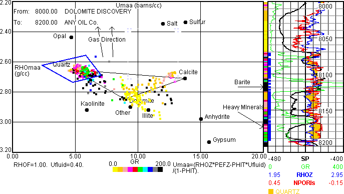
The RHOmaa-Umaa plot above suggests radioactive quartz (in blue polygon), calcite and dolomite are present with perhaps a little anhydrite or heavy mineral. Note the position of the M & M mineral mix called Other just below Dolomite. Other is a mixture of Dolomite and Clay and may be adjusted in JLog.
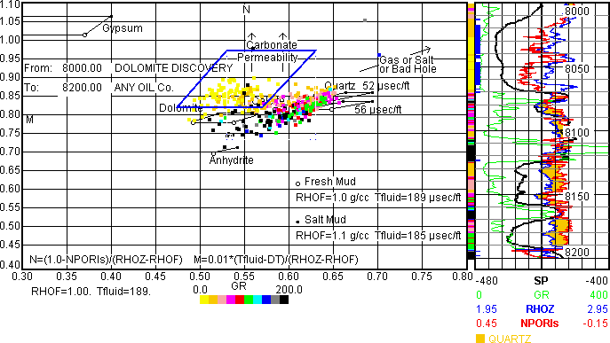
The MN plot above suggests permeable dolomite (in blue polygon) and the very high GR data is due to clay and shale. Quartz is somewhat radioactive in places. MN plots are very useful in identifying clays and shales as they stream to the lower left, often with increasing GR.
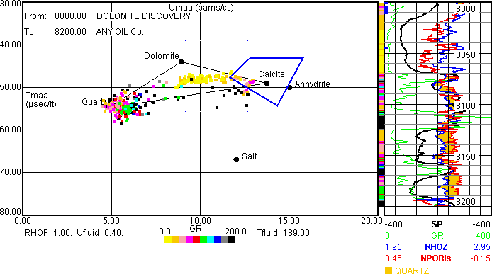
The Tmaa-Umaa plot above suggests radioactive quartz and clean dolomite and calcite are present. It appears the porous dolomite is capped by calcite (in blue polygon).
At this point lithology is established and it is evident that pay is present. The porosity and lithology logs appear to be well-calibrated.
Next some of the variables will be quantified and pay confirmed.
With Plots/Pickett/Pickett Porosity... select and push the "Density-Neutron" button. Check "Draw Pickett Plot Bulk Volume Water (BVW) lines.".
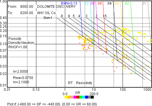
Then with Plots/Pickett/Pickett Plot... the Pickett Plot above (filtered on SP and GR) suggests Rw=0.075 (36,940 ppm NaCl) at 179.5 F at 8050 and m=2.10. Low Sw and low BVW confirm pay.
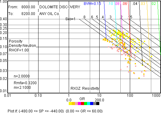
Changing Pickett RT to Rxo allows a check on Rmf and Archie porosity exponent m in the water zone. Rmf appears to be around 0.32 at reservoir temperature. This compares to Rmf=0.28 when the surface Rmf=0.748 at 63.5 F is converted to 179.5 F at 8050. m=2.10 appears to be reasonable.
With Models/Eval Mineral Models select 5-Mineral (carbonate + clay)... and leave default mineral values including TmaClay=65.0. Changing TmaClay will change Vclay and that may affect the Net Pay based on cutoff selection.
With Models/Eval Mineral Models/Porosity & Sw Models... select Density-Neutron porosity and Archie Sw.
Next, with Models/Eval Mineral Models/Porosity/Mineral Override... set Override 1 to 8190 - MDEPTH - 8201 - green - BAD HOLE and Constant porosity to 0.0. This will prevent a false show in bad hole.
With Models/Variables/a, m, n, Rw and Rmf... set a=1.0, m=2.1, n=2.0, Rw=0.075 and Rmf=0.32.
With Eval/Net Pay... use default cutoffs and oil for 40 acres drainage.
Eval/Calculate Quick Net Pay... From: 8000.0 To: 8200.0 yields 1,440,000 BBL OIL in place/40 acres at reservoir conditions for NPORls neutron.
After Eval/Paint Minerals and Fluids... we have the following with Eval/Plot Eval and 5 inch/100 ft (1/240)... From: 8000 To: 8200. Note the Anhydrite just below the pay that could also be a heavy mineral that sits right above the quartz sandstone (or chert). An examination of the cuttings might help here. Note also that Clay comes from the sonic-derived M & M model - not from the GR.

This workflow example demonstrates the steps one might make to evaluate DOLO.LAS.
Examples Extending JLog Features
Some JLog features can be expanded from their original purpose.
1: Porosity from GR
Here is an example making a shaly sand porosity estimate from the GR. First ADSscf, originally designed for estimating coal bed methane adsorbed gas will become the new GR porosity (GRpor) so it can be compared to PHIT density porosity. Then an evaluation will be made with density porosity and compared to the Function porosity made with GR.
JLog has a Function porosity model available for some Eval Mineral Models where a simple function is applied to a log curve to obtain porosity. The function needs to be defined.
Here, JLog is used to estimate shaly sand porosity from the Jackson #1 (from SAND.TXT) GR. This may be helpful when density log is missing or of poor quality. Calibration can be made in a key well and used elsewhere as needed.
After selecting Models/Eval Mineral Models/1-Mineral (clean or clayey)... select Density porosity with Models/Porosity & Sw Models... then with Models/Variables/Density Porosity... set RHOG=2.65 and RHOF=1.00. Do not correct Density Porosity for TOC. This sets the Calculated Curve PHIT to Density porosity.
With Plots/User/User Defined Plot... make the following two plots between PHIT (Y-axis) and GR (X-axis) from 4650-4850. Be sure to check the curve fit checkbox for each plot in order to obtain the function and correlation coefficient of the fit. And make sure Models/Eval Mineral Models/Porosity/Mineral Override... are turned off.
First, below, is a log-log PHIT vs. GR plot with PHIT from RHOB density porosity with RHOG=2.65 and RHOF=1.00 yielding a Power Curve Fit correlation coefficient=-0.78.

Next, below, is a linear-linear plot of the same data yielding a better Linear Curve Fit correlation coefficient=-0.80 for PHIT=0.2546 - 0.0016*GR. Thus a reasonable relationship exists between GR and PHIT (density porosity) for this shaly sand.

Now make a new Calculated Curve (GRpor) that estimates porosity from the GR. It will be compared to PHIT density porosity in track 2 below.
With Eval/Plot Which Calculated Curves?... select ADSscf, black, trk 2 and scale it 0.0 to 0.40. Then create a function called GRpor where a=0.2546 b= -0.0016*GR and c=1.0000. Select GR curve and rename GRpor instead of ADSscf.
Also select PHIT, red, trk 2 and scale it 0.0 to 0.40. PHIT at this point remains as Density porosity set up earlier. Both Calculated Curves are placed and compared in track 2 as below. Note how PHIT (density porosity) responds to the siderite streaks just above 4700 while GRpor does not.
Key variables are Rw=1.40, Rmf=0.45 and m=n=2.0. Vclay also comes from the GR with clean=8 and clay=105. Net Pay cutoffs are Vclay<0.50, PHIE>0.10 and Sw<0.50.

The Eval plot above with Density Porosity yields 3,016,000 BBL OIL/40 acres in place. VclayGR has been selected with GR clean: 8.00 and GR clay: 105 - this affects Net Pay cutoffs. PHIT in track 2 is Density porosity - compare it to GRpor.
Now make an evaluation with the above GR porosity function as follows: with Models/Porosity & Sw Models... select and push the "Function" button for Porosity Model and choose "GR" from the dropdown menu. Enter 0.2546 for a and -0.0016 for b and 1.0 for c just as for the GRpor Calculated Curve.
Key variables remain as Rw=1.40, Rmf=0.45 and m=n=2.0.

The Eval plot above with Function Porosity=0.2546 -0.0016*GR yields 2,480,000 BBL OIL/40 acres in place. PHIT in track 2 is now GR Function porosity and equals GRpor since both are computed with the same a, b and c parameters.
If GRpor looks strange be sure that Eval/Net Coal Gas Pay... "Dry As Free" and "Limit SCF/ton Gas to:" are not selected. You can get there after Models/Eval Mineral Models/Clay Rock Coal... .
Compare these to Example Evaluations / C: Clastic Reservoir results above that use same variables.
2: Compressional Sonic Travel Time (DTCO3) from Neutron Porosity (NPORls)
Suppose compressional sonic logs are needed to help calibrate a seismic study but sonic logs are in short supply and mainly density-neutron logs are available. NIOBRARA.JLG will be used as the calibration well to make a sonic log from a neutron log.
DTCO3 will be plotted (Y-axis) against NPORls (X-axis) in linear-linear scale as follows after opening NIOBRARA.JLG (shipped with JLog). This done with Plots/User/User Defined Plot... Be sure to check the Linear curve fit checkbox.
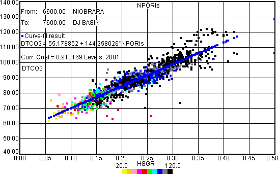
A reasonable relationship exists between DTCO3 and NPORls for this interval (6600-7600) where DTCO3=55.1789 + 144.2580*NPORls.
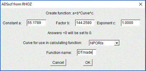
With Eval/Plot Which Calculated Curves?... select ADSscf and scale it 140 to 40 Blue color. Then create a function where a=55.1789 b=144.2580 and c=1.0000 as above. Select NPORls Curve from the drop down menu and name this new curve DTmade.
A log plot follows. Note how the new Calculated Curve called DTmade, in blue, falls right on top of the original black DTCO3 sonic over most of the interval. The above a, b and c values can be applied to similar neutron logs (scaled in limestone matrix porosity) over corresponding lithologic intervals in other wells, to generate a curve that minmics the sonic. The DTmade Calculated Curve can be saved, along with the logs, in TXT and LAS files to be imported by other software.
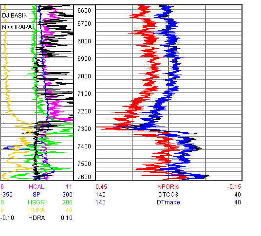
3: Adding Core and Other Data
Depth by Depth data such as core porosity can be added to a new column in a tab delimited text file saved from JLog, opened with a spreadsheet and re-imported to JLog.
Instructions can be found in JLog tips.doc shipped with JLog.
As an example four hypothetical core porosity values (CORPOR) are represented in black in track 3 below. Other data such as core Sw could be added in another column prior to re-import.
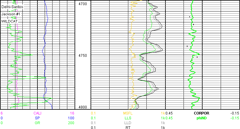
The above examples and workflows will get one aquainted with JLog. Much more is found in the Source & Tight Oil Manual 11.
JLog is a trademark of Bowler Petrophysics, Inc. Mac and Mac OS are trademarks of Apple Computer, Inc. Java is a trademark of Oracle Corporation. Windows is a trademark of Microsoft Corporation.
To order or for more information: contact Jack Bowler, Bowler Petrophysics, Inc., 730 17th Ave., Suite 835, Denver CO, 80202 USA. Phone: 303 860 1641. e-mail: jack@bowler-petrophysics.com.
Single JLog 11 license price is US $ 1,900.00 domestic and international. Handling, shipping and insurance charges depend on worldwide location. Customs, duty and brokerage fees are for the JLog recipient should they apply. Support is free by e-mail. No maintenance fee.
JLog is shipped on CD (or USB Flash Drive if no user CD drive is available) along with a USB port security key. Please keep the key in a safe place. If the key is lost so is JLog.
Payment is made in advance of shipment. If JLog does not solve your log analysis problems $1,900.00 will be refunded if JLog and the USB port security key are returned within 30 days.
Previous version users may upgrade to version 11. Contact Bowler Petrophysics for price that depends on present version. Handling, insurance and shipping charges depend on the ship to location. Previous version USB security keys will work with version 11. JLog 11 will read JLG files from all previous versions.
Numerous JLog features suggested by users and friends have been implemented - there are too many to mention but they know who they are and thank you for the suggestions.
Revised 31 January 2025.
